Note
Go to the end to download the full example code.
Regional model#
This example shows a simplified script for building a groundwater model in the northeast of the Netherlands. A primary feature of this area is an ice-pushed ridge called the Hondsrug. This examples demonstrates modifying external data for use in a MODFLOW 6 model.
In overview, the model features:
Thirteen layers: seven aquifers and six aquitards;
A dense ditch network in the east;
Pipe drainage for agriculture;
Precipitation and evapotranspiration.
We’ll start with the usual imports, and an import from scipy.
import matplotlib.pyplot as plt
import numpy as np
import pandas as pd
import scipy.ndimage
import xarray as xr

import imod
Before starting to create the input data, we will create the groundwater imod.mf6.GroundwaterFlowModel. The data from all the model packages will be added to this variable.
gwf_model = imod.mf6.GroundwaterFlowModel()
This package allows specifying a regular MODFLOW grid. This grid is assumed to be rectangular horizontally, but can be distorted vertically.
Load data#
We’ll load the data from the examples that come with this package.
layermodel = imod.data.hondsrug_layermodel()
# Make sure that the idomain is provided as integers
idomain = layermodel["idomain"].astype(int)
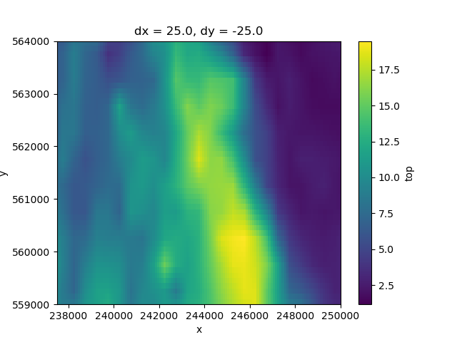
# We only need to provide the data for the top as a 2D array. MODFLOW 6 will
# compare the top against the uppermost active bottom cell.
top = layermodel["top"].max(dim="layer")
bot = layermodel["bottom"]
top.plot.imshow()
<matplotlib.image.AxesImage object at 0x0000019B381E5F40>
Adding information to the DIS package#
The following step is to add the previously created discretization data to the gwf_model variable. This is done using the function imod.mf6.StructuredDiscretization. The data to include is the top of the model domain, the bottom of the layers, and the idomain. All this information comes from the previously imported tifs (now converted to xarray.DataArray.
gwf_model["dis"] = imod.mf6.StructuredDiscretization(
    top=top, bottom=bot, idomain=idomain
)
Node property flow package - NPF#
This package contains the information related to the aquifer properties used to calculate hydraulic conductance. This package replaces the Layer Property Flow (LPF), Block-Centered Flow (BCF), and Upstream Weighting (UPW) packages from previous MODFLOW versions.
Hydraulic conductivity#
k = layermodel["k"]
icelltype#
The cell type to be used in the model (confined or convertible) can be defined under ICELLTYPE, which is an input to the NPF package. ICELLTYPE == 0: Confined cell - Constant transmissivity ICELLTYPE != 0: Convertible cell - Transmissivity varies depending on the calculated head in the cell (based on the saturated cell thickness)
In this example, all layers have a ICELLTYPE equal to 0, indicating confined cells. This is defined in the following section.
Adding information to the NPF package#
The information for the NPF package is added to the gwf_model variable using imod.mf6.NodePropertyFlow. The information included is the icelltype value (equal to zero), the array for the hydraulic conductivity (considered to be the same for the horizontal and vertical direction) and, optionally, the variable_vertical_conductance, dewatered, perched and save_flows options have been activated. For more details about the meaning of these variables and other variables available to be used within this package, please refer to the documentation.
gwf_model["npf"] = imod.mf6.NodePropertyFlow(
    icelltype=0,
    k=k,
    k33=k,
    variable_vertical_conductance=True,
    dewatered=True,
    perched=True,
    save_flows=True,
)
Initial conditions package - IC#
This package reads the starting heads for a simulation.
Starting heads interpolation#
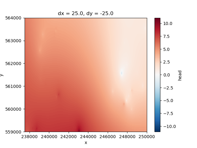
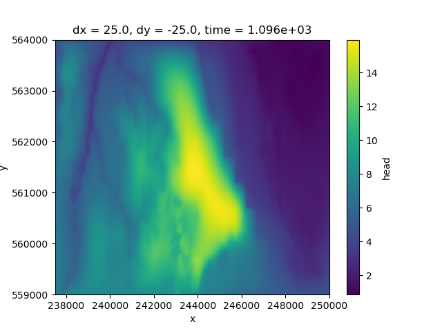
The starting heads to be used in this model are based on the interpolation of x-y head measurements, which were interpolated on a larger area. This example was created in this example –insert-link-here–
The heads were interpolated on a larger area, therefore these have to be clipped first
initial = imod.data.hondsrug_initial()
interpolated_head_larger = initial["head"]

xmin = 237_500.0
xmax = 250_000.0
ymin = 559_000.0
ymax = 564_000.0

interpolated_head = interpolated_head_larger.sel(
    x=slice(xmin, xmax), y=slice(ymax, ymin)
)

# Plotting the clipped interpolation
fig, ax = plt.subplots()
interpolated_head.plot.imshow(ax=ax)
<matplotlib.image.AxesImage object at 0x0000019B1C7434A0>
The final step is to assign the 2D heads interpolation to all the model layers (as a reference value) by using the xarray tool xarray.full_like. The 3d idomain array is used as reference for the geometry and then its original values are replaced by NaNs. This array is combined with the interpolated_head array using the xarray DataArray.combine_first option. The final result is an starting_heads xarray where all layers have the 2d interpolated_head information.
# Assign interpolated head values to all the model layers
like_3d = xr.full_like(idomain, np.nan, dtype=float)
starting_head = like_3d.combine_first(interpolated_head)
# Consequently ensure no data is specified in inactive cells:
starting_head = starting_head.where(idomain == 1)

starting_head
Adding information to the IC package#
The function for indicating the initial conditions is imod.mf6.InitialConditions. It is necessary to indicate the value(s) to be considered as the initial (starting) head of the simulation. In this case, this value is equal to the previously created starting_head array.
gwf_model["ic"] = imod.mf6.InitialConditions(starting_head)
Constant head package - CHD#
This package allows to indicate if the head varies with time, if it is constant or if it is inactive.
Constant head edge#
The previously interpolated starting_head array will be used to define the constant head value which will be used along the model boundaries. A function is defined to indicate the location of the outer edge (returning a boolean array).
def outer_edge(da):
    data = da.copy()
    from_edge = scipy.ndimage.binary_erosion(data)
    is_edge = (data == 1) & (from_edge == 0)
    return is_edge.astype(bool)
For the next calculations, it is necessary to create a template array which can be used for assigning the corresponding geometry to other arrays. In this case, a 2d template is created based on the idomain layer information and filled with ones.
like_2d = xr.full_like(idomain.isel(layer=0), 1)
like_2d
Using the previously created function and the 2d template, the outer edge is defined for this example.
edge = outer_edge(xr.full_like(like_2d.drop_vars("layer"), 1))
Adding information to the CHD package#
To add the information to the CHD package within the gwf_model variable, the imod.mf6.ConstantHead. function is used. The required information is the head array for this boundary condition. In this example, the starting_head array is selected where the idomain is > 0 (active) and it is located in the edge array.
It is also possible (and optional) to indicate if the CHD information will be written to the listing file after it is read (print_input), if the constant head flow rates will be printed to the listing file for every stress period time step in which “BUDGET PRINT” is specified in Output Control (print_flows) and if the constant head flow terms will be written to the file specified with “BUDGET FILEOUT” in Output Control (save_flows). By default, these three options are set to False.
gwf_model["chd"] = imod.mf6.ConstantHead(
    starting_head.where((idomain > 0) & edge),
    print_input=False,
    print_flows=True,
    save_flows=True,
)
Recharge#
This package is used to represent areally distributed recharge to the groundwater system. To calculate the recharge, the precipitation and evapotranspiration information from the KNMI website has been downloaded for the study area. This information is saved in netCDF files, which have been imported using the xarray function xr.open_dataset, slicing the area to the model’s miminum and maximum dimensions.
Note that the meteorological data has mm/d as unit and this has to be converted to m/d for MODFLOW 6.
xmin = 230_000.0
xmax = 257_000.0
ymin = 550_000.0
ymax = 567_000.0

meteorology = imod.data.hondsrug_meteorology()
pp = meteorology["precipitation"]
evt = meteorology["evapotranspiration"]

pp = pp.sel(x=slice(xmin, xmax), y=slice(ymax, ymin)) / 1000.0  # from mm/d to m/d
evt = evt.sel(x=slice(xmin, xmax), y=slice(ymax, ymin)) / 1000.0  # from mm/d to m/d
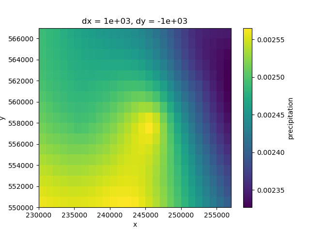
Recharge - Steady state#
For the steady state conditions of the model, the data from the period 2000 to 2009 was considered as reference. The initial information was sliced to this time period and averaged to obtain the a mean value grid. This process was done for both precipitation and evapotranspiration datasets.
Precipitation
pp_ss = pp.sel(time=slice("2000-01-01", "2009-12-31"))
pp_ss_mean = pp_ss.mean(dim="time")

fig, ax = plt.subplots()
pp_ss_mean.plot(ax=ax)
<matplotlib.collections.QuadMesh object at 0x0000019B382245F0>
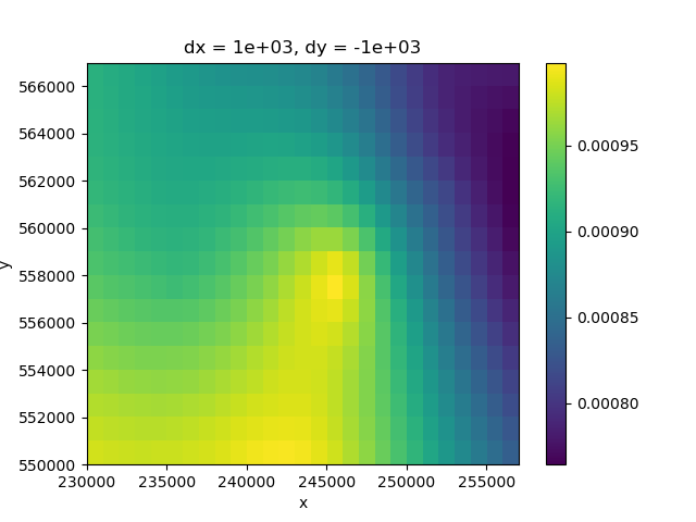
Evapotranspiration
evt_ss = evt.sel(time=slice("2000-01-01", "2009-12-31"))
evt_ss_mean = evt_ss.mean(dim="time")

fig, ax = plt.subplots()
evt_ss_mean.plot(ax=ax)

<matplotlib.collections.QuadMesh object at 0x0000019B242AB050>
For the recharge calculation, a first estimate is the difference between the precipitation and evapotranspiration values.
rch_ss = pp_ss_mean - evt_ss_mean

fig, ax = plt.subplots()
rch_ss.plot.imshow(ax=ax)
<matplotlib.image.AxesImage object at 0x0000019B39D25220>
Recharge - Transient#
The transient model will encompass the period from 2010 to 2015. The initial pp and evt datasets have been sliced to this time frame.
pp_trans = pp.sel(time=slice("2010-01-01", "2015-12-31"))
evt_trans = evt.sel(time=slice("2010-01-01", "2015-12-31"))
As previously done, it is assumed that the recharge is equal to the difference between precipitation and evapotranspiration as a first estimate. Furthermore, the negative values found after doing this calculation have been replaced by zeros, as the recharge should not have a negative value.
rch_trans = pp_trans - evt_trans
rch_trans = rch_trans.where(rch_trans > 0, 0)  # check negative values
The original information is on a daily step, so it is going to be resampled to a yearly step by using the xarray function Dataset.resample.
rch_trans_yr = rch_trans.resample(time="A", label="left").mean()
rch_trans_yr
To create the final recharge for the transient simulation, the steady state information needs to be concatenated to the transient recharge data. The steady state simulation will be run for one second. This is achieved by using the numpy Timedelta function, first creating a time delta of 1 second, which is assigned to the steady state recharge information. This dataset is then concatenated using the xarray function xarray.concat to the transient information and indicating that the dimension to join is “time”.
starttime = "2009-12-31"

# Add first steady-state
timedelta = np.timedelta64(1, "s")  # 1 second duration for initial steady-state
starttime_steady = np.datetime64(starttime) - timedelta
rch_ss = rch_ss.assign_coords(time=starttime_steady)

rch_ss_trans = xr.concat([rch_ss, rch_trans_yr], dim="time")
rch_ss_trans
The data obtained from KNMI has different grid dimensions than the one
considered in this example. To fix this, we’ll have to regrid the data to the
model grid. xugrid has Regridder functionality that allows to regrid data
with different methods. It is
also possible to define the regridding method such as nearest,
multilinear, mean, among others. In this case, mean was selected
and the 2d template (like_2d) was used as reference, as this is the geometry
to be considered in the model.
import xugrid as xu

regridder = xu.OverlapRegridder(rch_ss, like_2d, method="mean")
rch_ss_trans = regridder.regrid(rch_ss_trans)
rch_ss_trans
The previously created recharge array is a 2D array that needs to be assigned to a 3D array. This is done using the xarray DataArray.where option, where the recharge values are applied to the cells where the idomain value is larger than zero (that is, the active cells) and for the uppermost active cell (indicated by the minimum layer number).
rch_total = rch_ss_trans.where(
    idomain["layer"] == idomain["layer"].where(idomain > 0).min("layer")
)
rch_total
Finally, transposing the array dimensions using DataArray.transpose so they are in the correct order.
rch_total = rch_total.transpose("time", "layer", "y", "x")
rch_total

fig, ax = plt.subplots()
rch_total.isel(layer=2, time=6).plot.imshow(ax=ax)
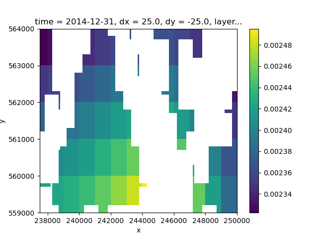
<matplotlib.image.AxesImage object at 0x0000019B1F052C60>
Adding information to the RCH package#
The information for the RCH package is added with the function imod.mf6.Recharge. It is required to insert the recharge flux rate, and it is optional to include the print_input, print_flows and save_flows information.
gwf_model["rch"] = imod.mf6.Recharge(rch_total)
Drainage package - DRN#
The drain package is used to simulate features that remove water from the aquifer, such as agricultural drains or springs. This occurs at a rate proportional to the head difference between the head in the aquifer and the drain elevation (the head in the aquifer has to be above that elevation). The conductance is the proportionality constant.
Import drainage information#
drainage = imod.data.hondsrug_drainage()

pipe_cond = drainage["conductance"]
pipe_elev = drainage["elevation"]

pipe_cond
Adding information to the DRN package#
To add the information to the DRN package within the gwf_model variable, the
imod.mf6.Drainage.
function is used. It is required to add the previously created arrays for
the drain elevation and the drain conductance.
It is optional to insert the information for
print_input, print_flows and save_flows
which are set to False by default.
gwf_model["drn-pipe"] = imod.mf6.Drainage(conductance=pipe_cond, elevation=pipe_elev)
River package - RIV#
This package simulates the effects of flow between surface-water features and groundwater systems.
Import river information#
river = imod.data.hondsrug_river()
riv_cond = river["conductance"]
riv_stage = river["stage"]
riv_bot = river["bottom"]
Adding information to the RIV package#
The data is assigned to the gwf_model variable by using imod.mf6.River, based on the previously imported conductance, stage and bottom arrays.
gwf_model["riv"] = imod.mf6.River(
    conductance=riv_cond, stage=riv_stage, bottom_elevation=riv_bot
)
Storage package - STO#
When the STO Package is included in a model, storage changes will be calculated, and thus, the model will be transient.
ss = 0.0003
layer = np.array([1, 2, 3, 4, 5, 6, 7, 8, 9, 10, 11, 12, 13])
sy = xr.DataArray(
    [0.16, 0.16, 0.16, 0.16, 0.15, 0.15, 0.15, 0.15, 0.14, 0.14, 0.14, 0.14, 0.14],
    {"layer": layer},
    ("layer",),
)
times_sto = np.array(
    [
        "2009-12-30T23:59:59.00",
        "2009-12-31T00:00:00.00",
        "2010-12-31T00:00:00.00",
        "2011-12-31T00:00:00.00",
        "2012-12-31T00:00:00.00",
        "2013-12-31T00:00:00.00",
        "2014-12-31T00:00:00.00",
    ],
    dtype="datetime64[ns]",
)

transient = xr.DataArray(
    [False, True, True, True, True, True, True], {"time": times_sto}, ("time",)
)
Adding information to the STO package#
The data is assigned to the gwf_model variable by using imod.mf6.SpecificStorage. It is necessary to indicate the values of specific storage, specific yield and if the layers are convertible.
gwf_model["sto"] = imod.mf6.SpecificStorage(
    specific_storage=ss,
    specific_yield=sy,
    transient=transient,
    convertible=0,
    save_flows=True,
)
Output Control package - OC#
This package determines how and when heads are printed to the listing file and/or written to a separate binary output file
Adding information to the OC package#
The function
imod.mf6.OutputControl
is used to store the information for this package.
It is possible to indicate if the heads and budget information is saved
at the end of each stress period (last),
for all timesteps a stress period (all),
or at the start of a stress period (first)
gwf_model["oc"] = imod.mf6.OutputControl(save_head="last", save_budget="last")
Model simulation#
In MODFLOW 6, the concept of “model” is that part of the program that solves a hydrologic process. MODFLOW 6 documentation supports one type of model: the GWF Model. It is possible within the MODFLOW 6 framewotk to solve multiple, tightly coupled, numerical models in a single system of equation, which may be multiple models of the same type or of different types.
The previously created gwf_model variable now contains the information from all the variables.
gwf_model
GroundwaterFlowModel(
    listing_file=None,
    print_input=False,
    print_flows=False,
    save_flows=False,
    newton=False,
    under_relaxation=False,
){
    'dis': StructuredDiscretization,
    'npf': NodePropertyFlow,
    'ic': InitialConditions,
    'chd': ConstantHead,
    'rch': Recharge,
    'drn-pipe': Drainage,
    'riv': River,
    'sto': SpecificStorage,
    'oc': OutputControl,
}
Attach the model information to a simulation#
The function imod.mf6.Modflow6Simulation allows to assign models to a simulation (in this case, the gwf_model).
simulation = imod.mf6.Modflow6Simulation("mf6-mipwa2-example")
simulation["GWF_1"] = gwf_model
Solver settings#
The solver settings are indicated using imod.mf6.Solution. If the values are not indicated manually, the defaults values will be considered.
simulation["solver"] = imod.mf6.Solution(
    modelnames=["GWF_1"],
    print_option="summary",
    outer_dvclose=1.0e-4,
    outer_maximum=500,
    under_relaxation=None,
    inner_dvclose=1.0e-4,
    inner_rclose=0.001,
    inner_maximum=100,
    linear_acceleration="cg",
    scaling_method=None,
    reordering_method=None,
    relaxation_factor=0.97,
)
Assign time discretization#
The time discretization of this model is 6 years.
simulation.create_time_discretization(
    additional_times=["2009-12-30T23:59:59.000000000", "2015-12-31T00:00:00.000000000"]
)
Run the model#
Note
The following lines assume the mf6 executable is available on your PATH.
The MODFLOW 6 examples introduction shortly
describes how to add it to yours.
modeldir = imod.util.temporary_directory()
simulation.write(modeldir, binary=False)
simulation.run()
Results visualization#
The next section indicated how to visualize the model results.
Import heads results#
The heads results are imported using imod.mf6.open_hds. on the background.
hds = simulation.open_head()
We can plot the data of an individual layer as follows
fig, ax = plt.subplots()
hds.sel(layer=3).isel(time=3).plot(ax=ax)
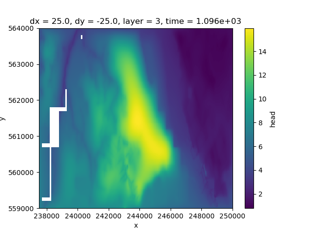
<matplotlib.collections.QuadMesh object at 0x0000019B2DCA31D0>
As you can see layer 3 has some missing cells in the west Whereas layer 4 only contains active cells in the eastern peatland area
fig, ax = plt.subplots()
hds.sel(layer=4).isel(time=3).plot(ax=ax)
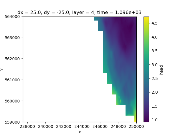
<matplotlib.collections.QuadMesh object at 0x0000019B2421A600>
Layer 5 contains more data towards the west, but has no active cells in the centre.
fig, ax = plt.subplots()
hds.sel(layer=5).isel(time=3).plot(ax=ax)
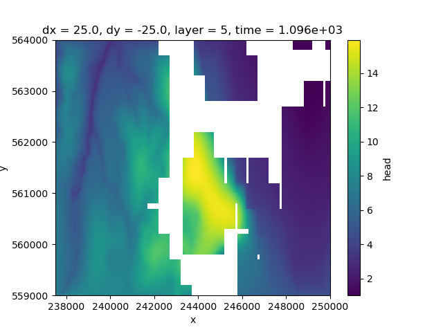
<matplotlib.collections.QuadMesh object at 0x0000019B35969430>
As you can see the data is individual layers have lots of inactive in different places.
It is difficult for this model to get a good idea what is happening across the area based on 1 layer alone. Luckily xarray allows us to compute the mean across a selection of layers and plot this.
By first selecting 3 layers with sel`,
and then computing the mean across the layer dimension
with mean(dim="layer").
fig, ax = plt.subplots()
hds.sel(layer=slice(3, 5)).mean(dim="layer").isel(time=3).plot(ax=ax)
<matplotlib.collections.QuadMesh object at 0x0000019B24218AD0>
Assign dates to head#
MODFLOW 6 has no concept of a calendar, so the output is not labelled only in terms of “time since start” in floating point numbers. For this model the time unit is days and we can assign a date coordinate as follows:
starttime = pd.to_datetime("2000-01-01")
timedelta = pd.to_timedelta(hds["time"], "D")
hds = hds.assign_coords(time=starttime + timedelta)
Extract head at points#
A typical operation is to extract simulated heads at point locations to compare them with measurements. In this example, we select the heads at two points:
x = [240_000.0, 244_000.0]
y = [560_000.0, 562_000.0]
selection = imod.select.points_values(hds, x=x, y=y)
The result can be converted into a pandas dataframe for timeseries analysis, or written to a variety of tabular file formats.
dataframe = selection.to_dataframe().reset_index()
dataframe = dataframe.rename(columns={"index": "id"})
dataframe
Total running time of the script: (2 minutes 25.441 seconds)