Hydrocoin

A 2D case from the Hydrological Code Intercomparison (Hydrocoin).

For more information see:

Konikow, L. F., Sanford, W. E., & Campbell, P. J. (1997). Constant-concentration boundary condition: Lessons from the HYDROCOIN variable-density groundwater benchmark problem. Water Resources Research, 33 (10), 2253-2261. https://doi.org/10.1029/97WR01926

import matplotlib.pyplot as plt

We’ll start with the usual imports

import numpy as np
import pandas as pd
import xarray as xr

import imod

Discretization

We’ll start off by creating a model discretization, since this is a simple conceptual model. The model is a 2D cross-section, hence nrow = 1.

nrow = 1  # number of rows
ncol = 45  # number of columns
nlay = 76  # number of layers

dz = 4.0
dx = 20.0
dy = -dx

Set up tops and bottoms

top1D = xr.DataArray(
    np.arange(nlay * dz, 0.0, -dz), {"layer": np.arange(1, nlay + 1)}, ("layer")
)

bot = top1D - dz

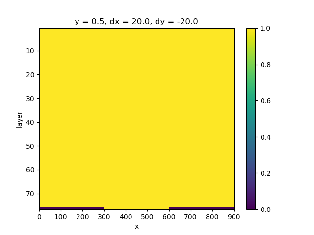
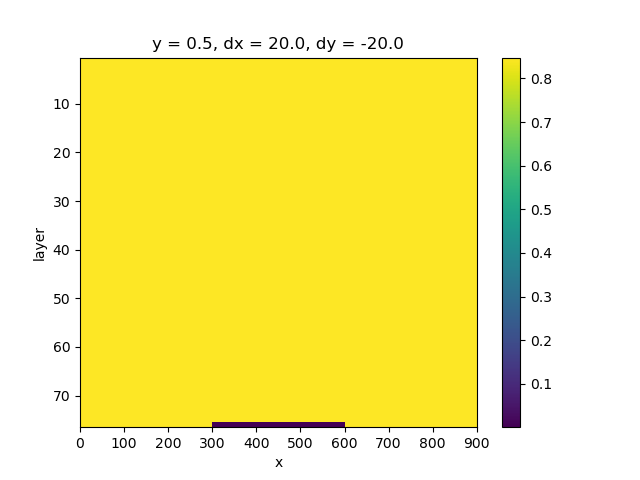
Set up ibound, which sets where active cells are (ibound = 1.0).

bnd = xr.DataArray(
    data=np.full((nlay, nrow, ncol), 1.0),
    coords={
        "y": [0.5],
        "x": np.arange(0.5 * dx, dx * ncol, dx),
        "layer": np.arange(1, 1 + nlay),
        "dx": dx,
        "dy": dy,
    },
    dims=("layer", "y", "x"),
)

Set inactive cells by specifying bnd[index] = 0.0

bnd[75, :, 0:15] = 0.0
bnd[75, :, 30:45] = 0.0

fig, ax = plt.subplots()
bnd.plot(y="layer", yincrease=False, ax=ax)

<matplotlib.collections.QuadMesh object at 0x00000204CEAEE910>

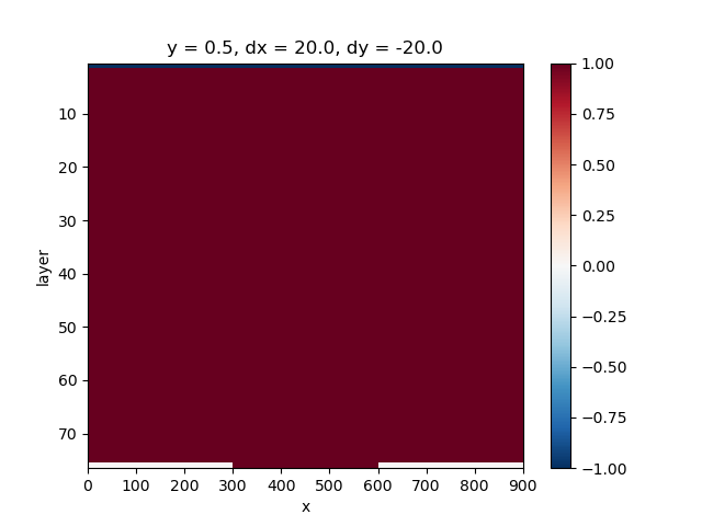
Boundary Conditions

Set the constant heads by specifying a negative value in iboud, that is: bnd[index] = -1

bnd[0, :, :] = -1


fig, ax = plt.subplots()
bnd.plot(y="layer", yincrease=False, ax=ax)

<matplotlib.collections.QuadMesh object at 0x00000204D7B0FD90>

Define WEL data, need to define the x, y, and pumping rate (q)

weldata = pd.DataFrame()
weldata["x"] = np.full(1, 0.5 * dx)
weldata["y"] = np.full(1, 0.5)
weldata["q"] = 0.28512  # positive, so it's an injection well

Define the icbund, which sets which cells in the solute transport model are active, inactive or constant.

In this case the central 15 cells on the top row have a constant concentration, And, on both sides, the outer 15 cells of the top row are inactive in the transport model.

icbund = xr.DataArray(
    data=np.full((nlay, nrow, ncol), 1.0),
    coords={
        "y": [0.5],
        "x": np.arange(0.5 * dx, dx * ncol, dx),
        "layer": np.arange(1, nlay + 1),
        "dx": dx,
        "dy": dy,
    },
    dims=("layer", "y", "x"),
)

icbund[75, :, 0:15] = 0.0
icbund[75, :, 30:45] = 0.0
icbund[75, :, 15:30] = -1.0

fig, ax = plt.subplots()
icbund.plot(y="layer", yincrease=False, ax=ax)

<matplotlib.collections.QuadMesh object at 0x00000204D97B8710>

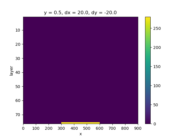
Initial conditions

Define the starting concentrations

sconc = xr.DataArray(
    data=np.full((nlay, nrow, ncol), 0.0),
    coords={
        "y": [0.5],
        "x": np.arange(0.5 * dx, dx * ncol, dx),
        "layer": np.arange(1, nlay + 1),
        "dx": dx,
        "dy": dy,
    },
    dims=("layer", "y", "x"),
)

sconc[75, :, 15:30] = 280.0

fig, ax = plt.subplots()
sconc.plot(y="layer", yincrease=False, ax=ax)

<matplotlib.collections.QuadMesh object at 0x00000204CDCD6B10>

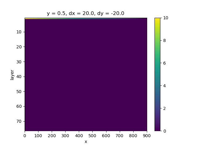
Define starting heads, these will be inserted in the Basic Flow (BAS) package

shd = xr.DataArray(
    data=np.full((nlay, nrow, ncol), 0.0),
    coords={
        "y": [0.5],
        "x": np.arange(0.5 * dx, dx * ncol, dx),
        "layer": np.arange(1, nlay + 1),
        "dx": dx,
        "dy": dy,
    },
    dims=("layer", "y", "x"),
)

shd[0, :, :] = np.array(
    [
        10,
        9.772727273,
        9.545454545,
        9.318181818,
        9.090909091,
        8.863636364,
        8.636363636,
        8.409090909,
        8.181818182,
        7.954545455,
        7.727272727,
        7.5,
        7.272727273,
        7.045454545,
        6.818181818,
        6.590909091,
        6.363636364,
        6.136363636,
        5.909090909,
        5.681818182,
        5.454545455,
        5.227272727,
        5,
        4.772727273,
        4.545454545,
        4.318181818,
        4.090909091,
        3.863636364,
        3.636363636,
        3.409090909,
        3.181818182,
        2.954545455,
        2.727272727,
        2.5,
        2.272727273,
        2.045454545,
        1.818181818,
        1.590909091,
        1.363636364,
        1.136363636,
        0.909090909,
        0.681818182,
        0.454545455,
        0.227272727,
        0.00,
    ]
)

fig, ax = plt.subplots()
shd.plot(y="layer", yincrease=False, ax=ax)

<matplotlib.collections.QuadMesh object at 0x00000204CE64D250>

Hydrogeology

Define horizontal hydraulic conductivity

khv = xr.DataArray(
    data=np.full((nlay, nrow, ncol), 0.847584),
    coords={
        "y": [0.5],
        "x": np.arange(0.5 * dx, dx * ncol, dx),
        "layer": np.arange(1, nlay + 1),
        "dx": dx,
        "dy": dy,
    },
    dims=("layer", "y", "x"),
)

khv[75, :, 15:30] = 0.0008475

fig, ax = plt.subplots()
khv.plot(y="layer", yincrease=False, ax=ax)

<matplotlib.collections.QuadMesh object at 0x00000204D9249F50>

Build

Finally, we build the model.

m = imod.wq.SeawatModel("Hydrocoin")
m["bas"] = imod.wq.BasicFlow(ibound=bnd, top=304.0, bottom=bot, starting_head=shd)
m["lpf"] = imod.wq.LayerPropertyFlow(
    k_horizontal=khv, k_vertical=khv, specific_storage=0.0
)
m["btn"] = imod.wq.BasicTransport(
    icbund=icbund, starting_concentration=sconc, porosity=0.2
)
m["adv"] = imod.wq.AdvectionTVD(courant=1.0)
m["dsp"] = imod.wq.Dispersion(longitudinal=20.0, diffusion_coefficient=0.0)
m["vdf"] = imod.wq.VariableDensityFlow(density_concentration_slope=0.71)
m["wel"] = imod.wq.Well(
    id_name="wel", x=weldata["x"], y=weldata["y"], rate=weldata["q"]
)
m["pcg"] = imod.wq.PreconditionedConjugateGradientSolver(
    max_iter=150, inner_iter=30, hclose=0.0001, rclose=0.1, relax=0.98, damp=1.0
)
m["gcg"] = imod.wq.GeneralizedConjugateGradientSolver(
    max_iter=150,
    inner_iter=30,
    cclose=1.0e-6,
    preconditioner="mic",
    lump_dispersion=True,
)
m["oc"] = imod.wq.OutputControl(save_head_idf=True, save_concentration_idf=True)
m.create_time_discretization(additional_times=["2000-01-01T00:00", "2010-01-01T00:00"])

Now we write the model, including runfile:

modeldir = imod.util.temporary_directory()
m.write(modeldir, resultdir_is_workdir=True)

Run

You can run the model using the comand prompt and the iMOD-WQ executable. This is part of the iMOD v5 release, which can be downloaded here: https://oss.deltares.nl/web/imod/download-imod5 . This only works on Windows.

To run your model, open up a command prompt and run the following commands:

cd c:\path\to\modeldir
c:\path\to\imod\folder\iMOD-WQ_V5_3_SVN359_X64R.exe Hydrocoin.run

Note that the version name of your executable might differ.

%% Visualise results —————–

After succesfully running the model, you can plot results as follows:

head = imod.idf.open(modeldir / "results/head/*.idf")

fig, ax = plt.subplots()
head.plot(yincrease=False, ax=ax)

conc = imod.idf.open(modeldir / "results/conc/*.idf")

fig, ax = plt.subplots()
conc.plot(levels=range(0, 35, 5), yincrease=False, ax=ax)