Different ways to regrid models

This example focuses on regridding. It uses the TWRI model from modflow6 (Harbaugh, 2005). More information about this model can be found in an example dedicated to building this model ( ex01_twri.py)

In overview, we’ll set the following steps: * we build a new grid, onto which we want to regrid the twri model * we regrid the model in 3 different ways ** first by regridding the simulation itself. This automatically regrids the model and all the packages in the model using default regridding methods for each field in each package ** second, we show how a model within a simulation can be regridded, also using default regridding methods ** third, we show how regridding can be done package per package. We illustrate that for one package, and we use a non-default regridding method for the horizontal conductivity field

We’ll start with the usual imports. As this is an simple (synthetic) structured model, we can make due with few packages.

import matplotlib.pyplot as plt
import numpy as np
import xarray as xr
from example_models import create_twri_simulation

from imod.mf6.regrid import NodePropertyFlowRegridMethod
from imod.mf6.utilities.regrid import RegridderType, RegridderWeightsCache

Now we create the twri simulation itself. It yields a simulation of a flow problem, with a grid of 3 layers and 15 cells in both x and y directions. To better illustrate the regridding, we replace the K field with a lognormal random K field. The original k-field is a constant per layer.

simulation = create_twri_simulation()

idomain = simulation["GWF_1"]["dis"]["idomain"]
heterogeneous_k = xr.zeros_like(idomain, dtype=np.double)
heterogeneous_k.values = np.random.lognormal(4.0, 1.0, heterogeneous_k.shape)
simulation["GWF_1"]["npf"]["k"] = heterogeneous_k

Let’s plot the k-field. This is going to be the input for the regridder, and the regridded output should somewhat resemble it.

fig, ax = plt.subplots()
heterogeneous_k.sel(layer=1).plot(y="y", yincrease=False, ax=ax)

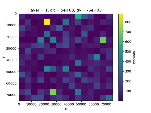
<matplotlib.collections.QuadMesh object at 0x00000204CDD83190>

Now we create a new grid for this simulation. It has 3 layers, 45 rows and 20 columns. The length of the domain is slightly different from the input grid. That had a coordinate difference between the first and last cellcentre on the x axis and y axis of 15*5000 = 75000 on both axes, but the new grid that is 75020 on the x axis and 75015 on the y axis

nlay = 3
nrow = 21
ncol = 12
shape = (nlay, nrow, ncol)

dx = 6251
dy = -3572
xmin = 0.0
xmax = dx * ncol
ymin = 0.0
ymax = abs(dy) * nrow
dims = ("layer", "y", "x")

layer = np.array([1, 2, 3])
y = np.arange(ymax, ymin, dy) + 0.5 * dy
x = np.arange(xmin, xmax, dx) + 0.5 * dx
coords = {"layer": layer, "y": y, "x": x, "dx": dx, "dy": dy}
target_grid = xr.DataArray(np.ones(shape, dtype=int), coords=coords, dims=dims)

A first way to regrid the twri model is to regrid the whole simulation object. This is the most straightforward method, and it uses default regridding methods for each input field. To see which ones are used, look at the _regrid_method class attribute of the relevant package. For example the _regrid_method attribute of the NodePropertyFlow package specifies that field “k” uses an OVERLAP regridder in combination with the averaging function “geometric_mean”.

new_simulation = simulation.regrid_like("regridded_twri", target_grid=target_grid)

Let’s plot the k-field. This is the regridded output, and it should should somewhat resemble the original k-field plotted earlier.

regridded_k_1 = new_simulation["GWF_1"]["npf"]["k"]
fig, ax = plt.subplots()
regridded_k_1.sel(layer=1).plot(y="y", yincrease=False, ax=ax)

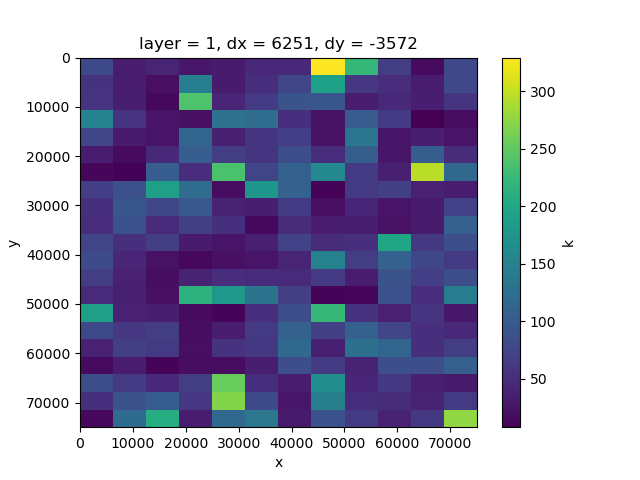
<matplotlib.collections.QuadMesh object at 0x00000204D1107950>

A second way to regrid twri is to regrid the groundwater flow model.

model = simulation["GWF_1"]
new_model = model.regrid_like(target_grid)

regridded_k_2 = new_model["npf"]["k"]
fig, ax = plt.subplots()
regridded_k_2.sel(layer=1).plot(y="y", yincrease=False, ax=ax)

<matplotlib.collections.QuadMesh object at 0x00000204CF387B90>

regridding method as well. in this example we’ll regrid the npf package manually and the rest of the packages using default methods.

Note that we create a RegridderWeightsCache here. This will store the weights of the regridder. Using the same cache to regrid another package will lead to a performance increase if that package uses the same regridding method, because initializing a regridder is costly.

regridder_types = NodePropertyFlowRegridMethod(k=(RegridderType.CENTROIDLOCATOR,))
regrid_context = RegridderWeightsCache()
npf_regridded = model["npf"].regrid_like(
    target_grid=target_grid,
    regrid_context=regrid_context,
    regridder_types=regridder_types,
)
new_model["npf"] = npf_regridded


regridded_k_3 = new_model["npf"]["k"]
fig, ax = plt.subplots()
regridded_k_3.sel(layer=1).plot(y="y", yincrease=False, ax=ax)

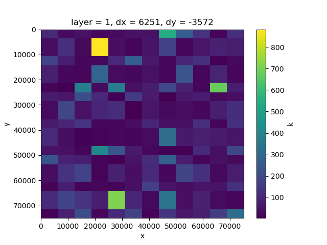
<matplotlib.collections.QuadMesh object at 0x00000204CF02D0D0>