Flow velocities and streamlines

In this section we will plot flow velocities and streamlines for some model results.

import matplotlib.pyplot as plt
import numpy as np
import xarray as xr

We’ll start with the usual imports

import imod

Load and unpack the data

ds_fluxes = imod.data.fluxes()
ds_fluxes = ds_fluxes.isel(time=-1)

ds_fluxes

lower = ds_fluxes["bdgflf"]
right = ds_fluxes["bdgfrf"]
front = ds_fluxes["bdgfff"]
heads = ds_fluxes["head"]

Calculating flow velocity

The imod-python function imod.evaluate.flow_velocity() computes flow velocities in m/d based on the budget results (bdgflf - flow lower face, bdgfrf - flow right face and bdgfff - flow front face). To apply this function, we first need to define a top_bot array.

top_bot = xr.full_like(lower, 1.0)
top_bot["top"] = top_bot["z"] - 0.5 * top_bot["dz"]
top_bot["bot"] = top_bot["z"] + 0.5 * top_bot["dz"]
top_bot

<xarray.DataArray 'bdgflf' (layer: 49, y: 218, x: 248)> Size: 11MB
array([[[1., 1., 1., ..., 1., 1., 1.],
        [1., 1., 1., ..., 1., 1., 1.],
        [1., 1., 1., ..., 1., 1., 1.],
        ...,
        [1., 1., 1., ..., 1., 1., 1.],
        [1., 1., 1., ..., 1., 1., 1.],
        [1., 1., 1., ..., 1., 1., 1.]],

       [[1., 1., 1., ..., 1., 1., 1.],
        [1., 1., 1., ..., 1., 1., 1.],
        [1., 1., 1., ..., 1., 1., 1.],
        ...,
        [1., 1., 1., ..., 1., 1., 1.],
        [1., 1., 1., ..., 1., 1., 1.],
        [1., 1., 1., ..., 1., 1., 1.]],

       [[1., 1., 1., ..., 1., 1., 1.],
        [1., 1., 1., ..., 1., 1., 1.],
        [1., 1., 1., ..., 1., 1., 1.],
        ...,
...
        ...,
        [1., 1., 1., ..., 1., 1., 1.],
        [1., 1., 1., ..., 1., 1., 1.],
        [1., 1., 1., ..., 1., 1., 1.]],

       [[1., 1., 1., ..., 1., 1., 1.],
        [1., 1., 1., ..., 1., 1., 1.],
        [1., 1., 1., ..., 1., 1., 1.],
        ...,
        [1., 1., 1., ..., 1., 1., 1.],
        [1., 1., 1., ..., 1., 1., 1.],
        [1., 1., 1., ..., 1., 1., 1.]],

       [[1., 1., 1., ..., 1., 1., 1.],
        [1., 1., 1., ..., 1., 1., 1.],
        [1., 1., 1., ..., 1., 1., 1.],
        ...,
        [1., 1., 1., ..., 1., 1., 1.],
        [1., 1., 1., ..., 1., 1., 1.],
        [1., 1., 1., ..., 1., 1., 1.]]], dtype=float32)
Coordinates:
  * x        (x) float64 2kB 9.095e+04 9.105e+04 ... 1.156e+05 1.156e+05
  * y        (y) float64 2kB 4.676e+05 4.674e+05 ... 4.46e+05 4.458e+05
    dx       float64 8B 100.0
    dy       float64 8B -100.0
    time     datetime64[ns] 8B 1979-12-31
  * layer    (layer) int32 196B 1 2 3 4 5 6 7 8 9 ... 41 42 43 44 45 46 47 48 49
    dz       (layer) float64 392B -2.0 -2.0 -2.0 -2.0 ... -10.0 -10.0 -10.0
    z        (layer) float64 392B 9.0 7.0 5.0 3.0 ... -225.0 -235.0 -245.0
    top      (layer) float64 392B 10.0 8.0 6.0 4.0 ... -220.0 -230.0 -240.0
    bot      (layer) float64 392B 8.0 6.0 4.0 2.0 ... -230.0 -240.0 -250.0

xarray.DataArray

'bdgflf'

• layer: 49
• y: 218
• x: 248

• 1.0 1.0 1.0 1.0 1.0 1.0 1.0 1.0 ... 1.0 1.0 1.0 1.0 1.0 1.0 1.0 1.0

  array([[[1., 1., 1., ..., 1., 1., 1.],
          [1., 1., 1., ..., 1., 1., 1.],
          [1., 1., 1., ..., 1., 1., 1.],
          ...,
          [1., 1., 1., ..., 1., 1., 1.],
          [1., 1., 1., ..., 1., 1., 1.],
          [1., 1., 1., ..., 1., 1., 1.]],
  
         [[1., 1., 1., ..., 1., 1., 1.],
          [1., 1., 1., ..., 1., 1., 1.],
          [1., 1., 1., ..., 1., 1., 1.],
          ...,
          [1., 1., 1., ..., 1., 1., 1.],
          [1., 1., 1., ..., 1., 1., 1.],
          [1., 1., 1., ..., 1., 1., 1.]],
  
         [[1., 1., 1., ..., 1., 1., 1.],
          [1., 1., 1., ..., 1., 1., 1.],
          [1., 1., 1., ..., 1., 1., 1.],
          ...,
  ...
          ...,
          [1., 1., 1., ..., 1., 1., 1.],
          [1., 1., 1., ..., 1., 1., 1.],
          [1., 1., 1., ..., 1., 1., 1.]],
  
         [[1., 1., 1., ..., 1., 1., 1.],
          [1., 1., 1., ..., 1., 1., 1.],
          [1., 1., 1., ..., 1., 1., 1.],
          ...,
          [1., 1., 1., ..., 1., 1., 1.],
          [1., 1., 1., ..., 1., 1., 1.],
          [1., 1., 1., ..., 1., 1., 1.]],
  
         [[1., 1., 1., ..., 1., 1., 1.],
          [1., 1., 1., ..., 1., 1., 1.],
          [1., 1., 1., ..., 1., 1., 1.],
          ...,
          [1., 1., 1., ..., 1., 1., 1.],
          [1., 1., 1., ..., 1., 1., 1.],
          [1., 1., 1., ..., 1., 1., 1.]]], dtype=float32)

• Coordinates: (10)
  • x
    (x)
    float64
    9.095e+04 9.105e+04 ... 1.156e+05

    array([ 90950.,  91050.,  91150., ..., 115450., 115550., 115650.])

  • y
    (y)
    float64
    4.676e+05 4.674e+05 ... 4.458e+05

    array([467550., 467450., 467350., ..., 446050., 445950., 445850.])

  • dx
    ()
    float64
    100.0

    array(100.)

  • dy
    ()
    float64
    -100.0

    array(-100.)

  • time
    ()
    datetime64[ns]
    1979-12-31

    array('1979-12-31T00:00:00.000000000', dtype='datetime64[ns]')

  • layer
    (layer)
    int32
    1 2 3 4 5 6 7 ... 44 45 46 47 48 49

    array([ 1,  2,  3,  4,  5,  6,  7,  8,  9, 10, 11, 12, 13, 14, 15, 16, 17, 18,
           19, 20, 21, 22, 23, 24, 25, 26, 27, 28, 29, 30, 31, 32, 33, 34, 35, 36,
           37, 38, 39, 40, 41, 42, 43, 44, 45, 46, 47, 48, 49], dtype=int32)

  • dz
    (layer)
    float64
    -2.0 -2.0 -2.0 ... -10.0 -10.0

    array([ -2.,  -2.,  -2.,  -2.,  -2.,  -2.,  -2.,  -2.,  -2.,  -2.,  -2.,
            -2.,  -2.,  -2.,  -2.,  -5.,  -5.,  -5.,  -5.,  -5.,  -5.,  -5.,
            -5.,  -5.,  -5.,  -5.,  -5.,  -5.,  -5.,  -5.,  -5.,  -5.,  -5.,
            -5.,  -5.,  -5.,  -5., -10., -10., -10., -10., -10., -10., -10.,
           -10., -10., -10., -10., -10.])

  • z
    (layer)
    float64
    9.0 7.0 5.0 ... -235.0 -245.0

    array([   9. ,    7. ,    5. ,    3. ,    1. ,   -1. ,   -3. ,   -5. ,
             -7. ,   -9. ,  -11. ,  -13. ,  -15. ,  -17. ,  -19. ,  -22.5,
            -27.5,  -32.5,  -37.5,  -42.5,  -47.5,  -52.5,  -57.5,  -62.5,
            -67.5,  -72.5,  -77.5,  -82.5,  -87.5,  -92.5,  -97.5, -102.5,
           -107.5, -112.5, -117.5, -122.5, -127.5, -135. , -145. , -155. ,
           -165. , -175. , -185. , -195. , -205. , -215. , -225. , -235. ,
           -245. ])

  • top
    (layer)
    float64
    10.0 8.0 6.0 ... -230.0 -240.0

    array([  10.,    8.,    6.,    4.,    2.,    0.,   -2.,   -4.,   -6.,
             -8.,  -10.,  -12.,  -14.,  -16.,  -18.,  -20.,  -25.,  -30.,
            -35.,  -40.,  -45.,  -50.,  -55.,  -60.,  -65.,  -70.,  -75.,
            -80.,  -85.,  -90.,  -95., -100., -105., -110., -115., -120.,
           -125., -130., -140., -150., -160., -170., -180., -190., -200.,
           -210., -220., -230., -240.])

  • bot
    (layer)
    float64
    8.0 6.0 4.0 ... -240.0 -250.0

    array([   8.,    6.,    4.,    2.,    0.,   -2.,   -4.,   -6.,   -8.,
            -10.,  -12.,  -14.,  -16.,  -18.,  -20.,  -25.,  -30.,  -35.,
            -40.,  -45.,  -50.,  -55.,  -60.,  -65.,  -70.,  -75.,  -80.,
            -85.,  -90.,  -95., -100., -105., -110., -115., -120., -125.,
           -130., -140., -150., -160., -170., -180., -190., -200., -210.,
           -220., -230., -240., -250.])

• Indexes: (3)
  • x
    PandasIndex

    PandasIndex(Index([ 90950.0,  91050.0,  91150.0,  91250.0,  91350.0,  91450.0,  91550.0,
            91650.0,  91750.0,  91850.0,
           ...
           114750.0, 114850.0, 114950.0, 115050.0, 115150.0, 115250.0, 115350.0,
           115450.0, 115550.0, 115650.0],
          dtype='float64', name='x', length=248))

  • y
    PandasIndex

    PandasIndex(Index([467550.0, 467450.0, 467350.0, 467250.0, 467150.0, 467050.0, 466950.0,
           466850.0, 466750.0, 466650.0,
           ...
           446750.0, 446650.0, 446550.0, 446450.0, 446350.0, 446250.0, 446150.0,
           446050.0, 445950.0, 445850.0],
          dtype='float64', name='y', length=218))

  • layer
    PandasIndex

    PandasIndex(Index([ 1,  2,  3,  4,  5,  6,  7,  8,  9, 10, 11, 12, 13, 14, 15, 16, 17, 18,
           19, 20, 21, 22, 23, 24, 25, 26, 27, 28, 29, 30, 31, 32, 33, 34, 35, 36,
           37, 38, 39, 40, 41, 42, 43, 44, 45, 46, 47, 48, 49],
          dtype='int32', name='layer'))

• Attributes: (0)

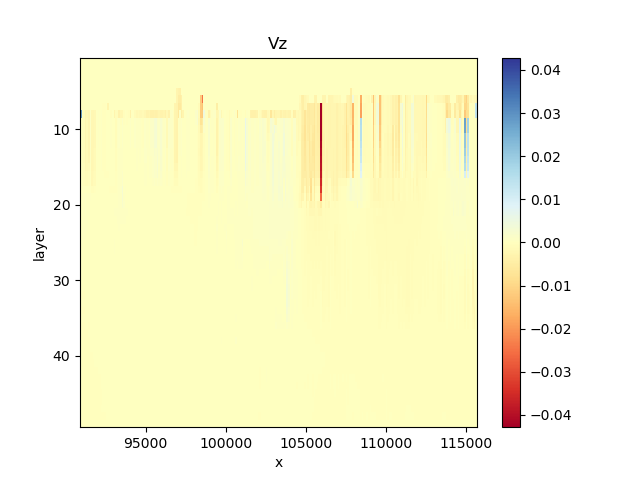
Next we’ll calculate the velocities and plot a cross-section of the vertical velocity at for y = 450050

fig, ax = plt.subplots()
vx, vy, vz = imod.evaluate.flow_velocity(
    front=front, lower=lower, right=right, top_bot=top_bot, porosity=0.3
)
vz.sel(y=450050.0, method="nearest").plot(cmap="RdYlBu", yincrease=False)

plt.title("Vz")

Text(0.5, 1.0, 'Vz')

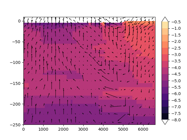
Quiver plot

It is also possible to make quiver plots for a cross section defined by two pairs of coordinates. We will first define arrays indicating the start and end location of the cross section to be evaluated.

start = np.array([97132.710, 457177.928])
end = np.array([103736.517, 457215.557])

Using the function imod.evaluate.quiver_line() considering the starting and ending points

u, v = imod.evaluate.quiver_line(right, front, lower, start, end)

Adding top and bottom information to the previously obtained arrays

u["top"] = u["z"] + 0.5 * u["dz"]
u["bottom"] = u["z"] - 0.5 * u["dz"]

v["top"] = v["z"] + 0.5 * v["dz"]
v["bottom"] = v["z"] - 0.5 * v["dz"]

Defining a cross section that shows the heads for the same location where the start and end points were defined, to use as a background image for the plot

cross_section = imod.select.cross_section_line(heads, start, end)
cross_section["top"] = cross_section["z"] - 0.5 * cross_section["dz"]
cross_section["bottom"] = cross_section["z"] + 0.5 * cross_section["dz"]

Ploting the cross section

colors = "magma"
levels = np.arange(-8, 0.0, 0.5)
skip = (slice(None, None, 2), slice(None, None, 2))
fig, ax = plt.subplots()
fig, ax = imod.visualize.cross_section(
    cross_section, colors=colors, levels=levels, ax=ax, fig=fig
)
imod.visualize.quiver(u[skip], v[skip], ax, kwargs_quiver={"color": "k"})

<matplotlib.quiver.Quiver object at 0x00000204CF027090>

Streamline function

This function shows the streamlines for a line cross section through a 3D flow field. We will use the previously created arrays that indicate the start and end location of the cross section and apply them in the function imod.evaluate.streamfunction_line()

streamfunction = imod.evaluate.streamfunction_line(right, front, start, end)

The previous array contains the streamfunction projected on the cross-section defined by provided linestring, with new dimension “s” along the cross-section. The cellsizes along “s” are given in the “ds” coordinate. The streamline function can be plotted using imod.visualize.streamfunction(), but first we need to define the ‘top’ and ‘bottom’ of the layers in the array Note: By default the steamlines are plotted in white.

streamfunction["bottom"] = streamfunction["z"] + streamfunction["dz"]
streamfunction["top"] = streamfunction["z"]

fig, ax = plt.subplots()
fig, ax = imod.visualize.cross_section(
    cross_section, colors=colors, levels=levels, ax=ax, fig=fig
)
imod.visualize.streamfunction(streamfunction, ax=ax, n_streamlines=10)

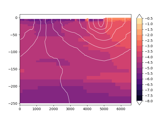
<matplotlib.contour.QuadContourSet object at 0x00000204D97A6050>