1D Solute Transport Benchmarks

This example is taken from the MODFLOW6 Examples, number 35.

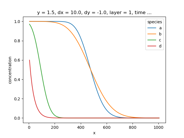
As explained there, the setup is a simple 1d homogeneous aquifer with a steady state flow field of constant velocity. The benchmark consists of four transport problems that are modeled using this flow field. Here we have modeled these four transport problems as a single simulation with multiple species. In all cases the initial concentration in the domain is zero, but water entering the domain has a concentration of one:

• species a is transported with zero diffusion or dispersion and the concentration distribution should show a sharp front, but due to the numerical method we see some smearing, which is expected.

• species b has a sizeable dispersivity and hence shows more smearing than species a but the same centre of mass.

• Species c has linear sorption and therefore the concentration doesn’t enter the domain as far as species a or species b, but the front of the solute plume has the same overall shape as for species a or species b.

• Species d has linear sorption and first order decay, and this changes the shape of the front of the solute plume.

import numpy as np
import pandas as pd
import xarray as xr

import imod


def create_transport_model(flowmodel, speciesname, dispersivity, retardation, decay):
    """
    Function to create a transport model, as we intend to create four similar
    transport models.

    Parameters
    ----------
    flowmodel: GroundwaterFlowModel
    speciesname: str
    dispersivity: float
    retardation: float
    decay: float

    Returns
    -------
    transportmodel: GroundwaterTransportModel
    """

    rhobulk = 1150.0
    porosity = 0.25

    tpt_model = imod.mf6.GroundwaterTransportModel()
    tpt_model["ssm"] = imod.mf6.SourceSinkMixing.from_flow_model(
        flowmodel, speciesname, save_flows=True
    )
    tpt_model["adv"] = imod.mf6.AdvectionUpstream()
    tpt_model["dsp"] = imod.mf6.Dispersion(
        diffusion_coefficient=0.0,
        longitudinal_horizontal=dispersivity,
        transversal_horizontal1=0.0,
        xt3d_off=False,
        xt3d_rhs=False,
    )

    # Compute the sorption coefficient based on the desired retardation factor
    # and the bulk density. Because of this, the exact value of bulk density
    # does not matter for the solution.
    if retardation != 1.0:
        sorption = "linear"
        kd = (retardation - 1.0) * porosity / rhobulk
    else:
        sorption = None
        kd = 1.0

    tpt_model["mst"] = imod.mf6.MobileStorageTransfer(
        porosity=porosity,
        decay=decay,
        decay_sorbed=decay,
        bulk_density=rhobulk,
        distcoef=kd,
        first_order_decay=True,
        sorption=sorption,
    )

    tpt_model["ic"] = imod.mf6.InitialConditions(start=0.0)
    tpt_model["oc"] = imod.mf6.OutputControl(
        save_concentration="all", save_budget="last"
    )
    tpt_model["dis"] = flowmodel["dis"]
    return tpt_model

Create the spatial discretization.

nlay = 1
nrow = 2
ncol = 101
dx = 10.0
xmin = 0.0
xmax = dx * ncol
layer = [1]
y = [1.5, 0.5]
x = np.arange(xmin, xmax, dx) + 0.5 * dx

grid_dims = ("layer", "y", "x")
grid_coords = {"layer": layer, "y": y, "x": x}
grid_shape = (nlay, nrow, ncol)
grid = xr.DataArray(np.ones(grid_shape, dtype=int), coords=grid_coords, dims=grid_dims)
bottom = xr.full_like(grid, -1.0, dtype=float)

gwf_model = imod.mf6.GroundwaterFlowModel()
gwf_model["ic"] = imod.mf6.InitialConditions(0.0)

Create the input for a constant head boundary and its associated concentration.

constant_head = xr.full_like(grid, np.nan, dtype=float)
constant_head[..., 0] = 60.0
constant_head[..., 100] = 0.0

constant_conc = xr.full_like(grid, np.nan, dtype=float)
constant_conc[..., 0] = 1.0
constant_conc[..., 100] = 0.0
constant_conc = constant_conc.expand_dims(
    species=["species_a", "species_b", "species_c", "species_d"]
)

gwf_model["chd"] = imod.mf6.ConstantHead(constant_head, constant_conc)

Add other flow packages.

gwf_model["npf"] = imod.mf6.NodePropertyFlow(
    icelltype=1,
    k=xr.full_like(grid, 1.0, dtype=float),
    variable_vertical_conductance=True,
    dewatered=True,
    perched=True,
)
gwf_model["dis"] = imod.mf6.StructuredDiscretization(
    top=0.0,
    bottom=bottom,
    idomain=grid,
)
gwf_model["oc"] = imod.mf6.OutputControl(save_head="all", save_budget="all")
gwf_model["sto"] = imod.mf6.SpecificStorage(
    specific_storage=1.0e-5,
    specific_yield=0.15,
    transient=False,
    convertible=0,
)

Create the simulation.

simulation = imod.mf6.Modflow6Simulation("1d_tpt_benchmark")
simulation["flow"] = gwf_model

Add four transport simulations, and setup the solver flow and transport.

simulation["tpt_a"] = create_transport_model(gwf_model, "species_a", 0.0, 1.0, 0.0)
simulation["tpt_b"] = create_transport_model(gwf_model, "species_b", 10.0, 1.0, 0.0)
simulation["tpt_c"] = create_transport_model(gwf_model, "species_c", 10.0, 5.0, 0.0)
simulation["tpt_d"] = create_transport_model(gwf_model, "species_d", 10.0, 5.0, 0.002)

simulation["flow_solver"] = imod.mf6.Solution(
    modelnames=["flow"],
    print_option="summary",
    outer_dvclose=1.0e-4,
    outer_maximum=500,
    under_relaxation=None,
    inner_dvclose=1.0e-4,
    inner_rclose=0.001,
    inner_maximum=100,
    linear_acceleration="bicgstab",
    scaling_method=None,
    reordering_method=None,
    relaxation_factor=0.97,
)
simulation["transport_solver"] = imod.mf6.Solution(
    modelnames=["tpt_a", "tpt_b", "tpt_c", "tpt_d"],
    print_option="summary",
    outer_dvclose=1.0e-4,
    outer_maximum=500,
    under_relaxation=None,
    inner_dvclose=1.0e-4,
    inner_rclose=0.001,
    inner_maximum=100,
    linear_acceleration="bicgstab",
    scaling_method=None,
    reordering_method=None,
    relaxation_factor=0.97,
)

duration = pd.to_timedelta("2000d")
start = pd.to_datetime("2000-01-01")
simulation.create_time_discretization(additional_times=[start, start + duration])
simulation["time_discretization"]["n_timesteps"] = 100

Run the simulation.

modeldir = imod.util.temporary_directory()
simulation.write(modeldir, binary=False)
simulation.run()

Open the concentration results and store them in a single DataArray.

concentration = simulation.open_concentration(species_ls=["a", "b", "c", "d"])
mass_budgets = simulation.open_transport_budget(species_ls=["a", "b", "c", "d"])

Visualize the last concentration profiles of the model run for the different species.

concentration.isel(time=-1, y=0).plot(x="x", hue="species")

[<matplotlib.lines.Line2D object at 0x00000204CF0E41D0>, <matplotlib.lines.Line2D object at 0x00000204CF0F3010>, <matplotlib.lines.Line2D object at 0x00000204CBDE3C90>, <matplotlib.lines.Line2D object at 0x00000204CD812C10>]