Lake package example

This is a synthetic example (using invented, not necesarily physical data) of how to use the lake package api to generate models with lakes.

In overview, we’ll set the following steps:

• Create a structured grid for a rectangular geometry.

• Create a constant head boundary

• Create packages for initial conditions, output control, storage, and node property flow

• Create a lake package with a time-dependent rainfall

• Write to modflow6 files.

• Run the model.

• Open the results back into DataArrays.

• Visualize the results.

We’ll start with the usual imports. As this is an simple (synthetic) structured model, we can make due with few packages.

import numpy as np
import xarray as xr

import imod
import imod.mf6.lak as lak

nlay = 3
nrow = 15
ncol = 15
shape = (nlay, nrow, ncol)

dx = 5000.0
dy = -5000.0
xmin = 0.0
xmax = dx * ncol
ymin = 0.0
ymax = abs(dy) * nrow
dims = ("layer", "y", "x")

layer = np.array([1, 2, 3])
y = np.arange(ymax, ymin, dy) + 0.5 * dy
x = np.arange(xmin, xmax, dx) + 0.5 * dx
coords = {"layer": layer, "y": y, "x": x}

idomain = xr.DataArray(np.ones(shape, dtype=int), coords=coords, dims=dims)

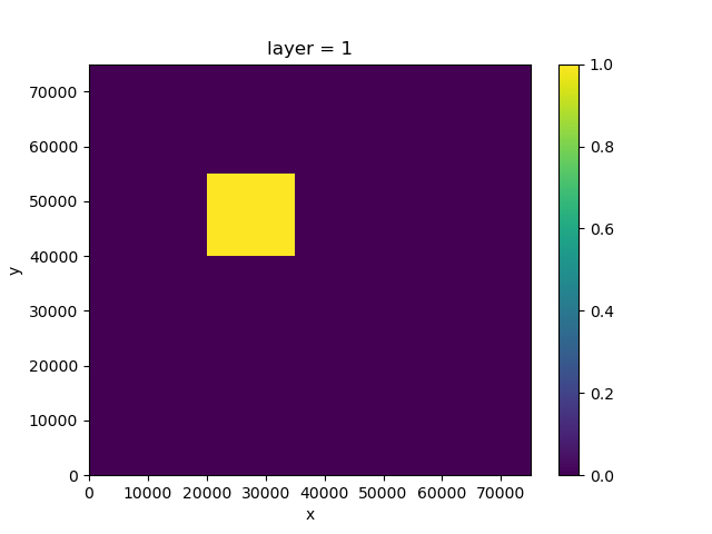
lake_layer = 1
lake_x = x[4:7]
lake_y = y[4:7]
is_lake = xr.full_like(idomain, fill_value=False, dtype=bool)
is_lake.loc[{"layer": lake_layer, "x": lake_x, "y": lake_y}] = True
is_lake.sel(layer=1).plot.imshow()

<matplotlib.image.AxesImage object at 0x00000204CED41A10>

VERTICAL = 1
connectionType = xr.where(is_lake, VERTICAL, np.nan)
bed_leak = xr.where(is_lake, 0.2, np.nan)
top_elevation = xr.where(is_lake, 0.4, np.nan)
bot_elevation = xr.where(is_lake, 0.1, np.nan)
connection_length = xr.where(is_lake, 0.5, np.nan)
connection_width = xr.where(is_lake, 0.6, np.nan)

times_rainfall = [
    np.datetime64("2000-01-01"),
    np.datetime64("2000-03-01"),
    np.datetime64("2000-05-01"),
]

rainfall = xr.DataArray(
    np.full((len(times_rainfall)), 0.001),
    coords={"time": times_rainfall},
    dims=["time"],
)


lake = lak.LakeData(
    10.0,
    "Nieuwkoopse_plas",
    connectionType,
    bed_leak,
    top_elevation,
    bot_elevation,
    connection_length,
    connection_width,
    None,
    None,
    rainfall,
    None,
    None,
    None,
    None,
    None,
)

C:\buildagent\work\4b9080cbb3354582\imod-python\examples\mf6\lake.py:74: UserWarning: Converting non-nanosecond precision datetime values to nanosecond precision. This behavior can eventually be relaxed in xarray, as it is an artifact from pandas which is now beginning to support non-nanosecond precision values. This warning is caused by passing non-nanosecond np.datetime64 or np.timedelta64 values to the DataArray or Variable constructor; it can be silenced by converting the values to nanosecond precision ahead of time.
  rainfall = xr.DataArray(

Create grid coordinates

The first steps consist of setting up the grid – first the number of layer, rows, and columns. Cell sizes are constant throughout the model.

We’ll create a new directory in which we will write and run the model.

modeldir = imod.util.temporary_directory()

Create DataArrays

Now that we have the grid coordinates setup, we can start defining model parameters. The model is characterized by:

• a constant head boundary on the left

• a single drain in the center left of the model

• uniform recharge on the top layer

bottom = xr.DataArray([-200.0, -300.0, -450.0], {"layer": layer}, ("layer",))

# Constant head
constant_head = xr.full_like(idomain, np.nan, dtype=float).sel(layer=[1, 2])
constant_head[..., 0] = 0.0

# Node properties
icelltype = xr.DataArray([1, 0, 0], {"layer": layer}, ("layer",))
k = xr.DataArray([1.0e-3, 1.0e-4, 2.0e-4], {"layer": layer}, ("layer",))
k33 = xr.DataArray([2.0e-8, 2.0e-8, 2.0e-8], {"layer": layer}, ("layer",))

gwf_model = imod.mf6.GroundwaterFlowModel()
gwf_model["dis"] = imod.mf6.StructuredDiscretization(
    top=200.0, bottom=bottom, idomain=idomain
)
gwf_model["chd"] = imod.mf6.ConstantHead(
    constant_head, print_input=True, print_flows=True, save_flows=True
)
gwf_model["ic"] = imod.mf6.InitialConditions(head=0.0)
gwf_model["npf"] = imod.mf6.NodePropertyFlow(
    icelltype=icelltype,
    k=k,
    k33=k33,
    variable_vertical_conductance=True,
    dewatered=True,
    perched=True,
    save_flows=True,
)
gwf_model["sto"] = imod.mf6.SpecificStorage(
    specific_storage=1.0e-5,
    specific_yield=0.15,
    transient=True,
    convertible=0,
)
gwf_model["oc"] = imod.mf6.OutputControl(save_head="all", save_budget="all")

# Attach it to a simulation
simulation = imod.mf6.Modflow6Simulation("ex01-twri")
simulation["GWF_1"] = gwf_model
# Define solver settings
simulation["solver"] = imod.mf6.Solution(
    modelnames=["GWF_1"],
    print_option="summary",
    outer_dvclose=1.0e-4,
    outer_maximum=500,
    under_relaxation=None,
    inner_dvclose=1.0e-4,
    inner_rclose=0.001,
    inner_maximum=100,
    linear_acceleration="cg",
    scaling_method=None,
    reordering_method=None,
    relaxation_factor=0.97,
)

gwf_model["lake"] = lak.Lake.from_lakes_and_outlets(
    [lake],
    print_input=True,
    print_stage=True,
    print_flows=True,
    save_flows=True,
    stagefile=modeldir / "GWF_1/stagefile.lak",
    budgetcsvfile=modeldir / "GWF_1/budgetcsvfile.lak",
    package_convergence_filename=modeldir / "GWF_1/convergence.lak",
)

# Collect time discretization
simulation.create_time_discretization(
    additional_times=["2000-01-01", "2000-01-02", "2000-01-03", "2013-06-04"]
)


simulation.write(modeldir)

Run the model

Note

The following lines assume the mf6 executable is available on your PATH. The Modflow 6 examples introduction shortly describes how to add it to yours.

simulation.run()

Open the results

We’ll open the heads (.hds) file.

head = imod.mf6.open_hds(
    modeldir / "GWF_1/GWF_1.hds",
    modeldir / "GWF_1/dis.dis.grb",
)

Visualize the results

head.isel(layer=0, time=4).plot.contourf()

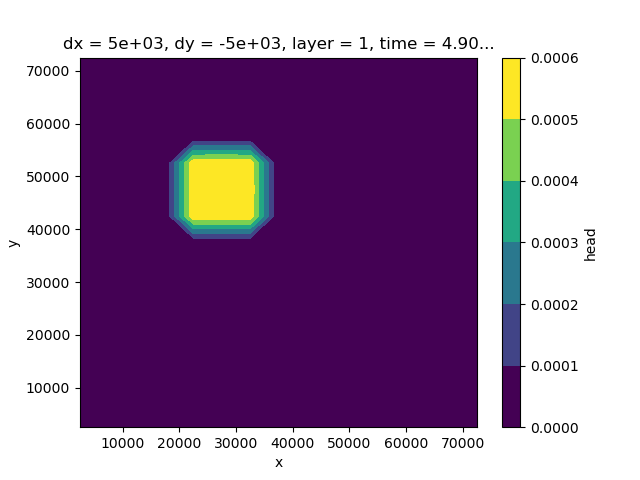
<matplotlib.contour.QuadContourSet object at 0x00000204CF00A990>