Saltwater Pocket

This 2D example demonstrates the development of a saltwater pocket in a fresh groundwater environment.

import matplotlib.pyplot as plt

import numpy as np
import xarray as xr

import imod

We’ll start with the usual imports

nrow = 1  # number of rows
ncol = 80  # number of column
nlay = 40  # number of layers

dz = 1.0  # 0.0125
dx = 1.0  # 0.0125
dy = -dx

Setup tops and bottoms

top1D = xr.DataArray(
    np.arange(nlay * dz, 0.0, -dz), {"layer": np.arange(1, nlay + 1)}, ("layer")
)

bot = top1D - dz

Set up ibound, which sets where active cells are (ibound = 1.0)

bnd = xr.DataArray(
    data=np.full((nlay, nrow, ncol), 1.0),
    coords={
        "y": [0.5],
        "x": np.arange(0.5 * dx, dx * ncol, dx),
        "layer": np.arange(1, 1 + nlay),
        "dx": dx,
        "dy": dy,
    },
    dims=("layer", "y", "x"),
)

fig, ax = plt.subplots()
bnd.plot(y="layer", yincrease=False, ax=ax)

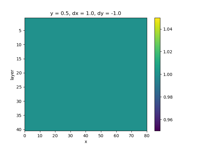
<matplotlib.collections.QuadMesh object at 0x00000204CF37BE10>

Boundary Conditions

Set the constant heads by specifying a negative value in iboud, that is: bnd[index] = -1`

bnd[21, :, 0] = -1

Initial Conditions

Define the starting concentration

sconc = xr.DataArray(
    data=np.full((nlay, nrow, ncol), 0.0),
    coords={
        "y": [0.5],
        "x": np.arange(0.5 * dx, dx * ncol, dx),
        "layer": np.arange(1, nlay + 1),
    },
    dims=("layer", "y", "x"),
)

sconc[16:24, :, 41:80] = 35.0

fig, ax = plt.subplots()
sconc.plot(y="layer", yincrease=False, ax=ax)

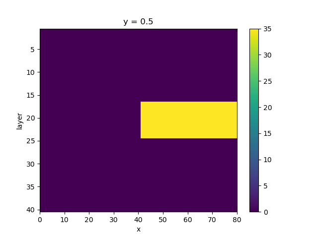
<matplotlib.collections.QuadMesh object at 0x00000204D6C7EFD0>

Build

Finally, we build the model.

m = imod.wq.SeawatModel("SaltwaterPocket")
m["bas"] = imod.wq.BasicFlow(ibound=bnd, top=40, bottom=bot, starting_head=0.0)
m["lpf"] = imod.wq.LayerPropertyFlow(
    k_horizontal=86.4, k_vertical=86.4, specific_storage=0.0
)
m["btn"] = imod.wq.BasicTransport(
    icbund=bnd, starting_concentration=sconc, porosity=0.1
)
m["adv"] = imod.wq.AdvectionTVD(courant=1.0)
m["dsp"] = imod.wq.Dispersion(longitudinal=0.001, diffusion_coefficient=0.0000864)
m["vdf"] = imod.wq.VariableDensityFlow(density_concentration_slope=0.71)
m["wel"] = imod.wq.Well(id_name="wel", x=0.5 * dx, y=0.5, rate=0.28512)
m["pcg"] = imod.wq.PreconditionedConjugateGradientSolver(
    max_iter=150, inner_iter=30, hclose=0.0001, rclose=0.1, relax=0.98, damp=1.0
)
m["gcg"] = imod.wq.GeneralizedConjugateGradientSolver(
    max_iter=150,
    inner_iter=30,
    cclose=1.0e-6,
    preconditioner="mic",
    lump_dispersion=True,
)
m["oc"] = imod.wq.OutputControl(save_head_idf=True, save_concentration_idf=True)
m.create_time_discretization(additional_times=["2000-01-01T00:00", "2000-01-05T01:00"])

Now we write the model, including runfile:

modeldir = imod.util.temporary_directory()
m.write(modeldir, resultdir_is_workdir=True)

Run

You can run the model using the comand prompt and the iMOD-WQ executable. This is part of the iMOD v5 release, which can be downloaded here: https://oss.deltares.nl/web/imod/download-imod5 . This only works on Windows.

To run your model, open up a command prompt and run the following commands:

cd c:\path\to\modeldir
c:\path\to\imod\folder\iMOD-WQ_V5_3_SVN359_X64R.exe SaltwaterPocket.run

Note that the version name of your executable might differ.

Visualise results

After succesfully running the model, you can plot results as follows:

head = imod.idf.open(modeldir / "results/head/*.idf")

fig, ax = plt.subplots()
head.plot(yincrease=False, ax=ax)

conc = imod.idf.open(modeldir / "results/conc/*.idf")

fig, ax = plt.subplots()
conc.plot(levels=range(0, 35, 5), yincrease=False, ax=ax)

%%