Circle

This example illustrates how to setup a very simple unstructured groundwater model using the imod package and associated packages.

In overview, we’ll set the following steps:

• Create a triangular mesh for a disk geometry.

• Create the xugrid UgridDataArrays containg the MODFLOW6 parameters.

• Feed these arrays into the imod mf6 classes.

• Write to modflow6 files.

• Run the model.

• Open the results back into UgridDataArrays.

• Visualize the results.

We’ll start with the following imports:

import matplotlib.pyplot as plt
import numpy as np
import xarray as xr
import xugrid as xu
from pandas import isnull

import imod

Create a mesh

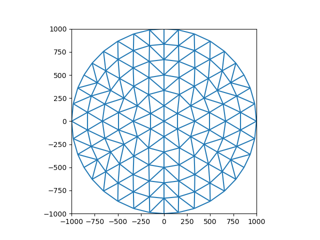
The first steps consists of generating a mesh. In this example, we’ll use data included with iMOD Python for a circular mesh. Note that this is a Ugrid2D object. For more information on working with unstructured grids see the Xugrid documentation

grid = imod.data.circle()

grid

<xarray.Dataset> Size: 10kB
Dimensions:            (mesh2d_nFaces: 216, mesh2d_nMax_face_nodes: 3,
                        mesh2d_nEdges: 342, two: 2, mesh2d_nNodes: 127)
Coordinates:
    mesh2d_node_x      (mesh2d_nNodes) float64 1kB 0.0 6.123e-14 ... 331.1 157.5
    mesh2d_node_y      (mesh2d_nNodes) float64 1kB 0.0 1e+03 ... 764.7 818.3
Dimensions without coordinates: mesh2d_nFaces, mesh2d_nMax_face_nodes,
                                mesh2d_nEdges, two, mesh2d_nNodes
Data variables:
    mesh2d             int32 4B 0
    mesh2d_face_nodes  (mesh2d_nFaces, mesh2d_nMax_face_nodes) int32 3kB 0 ... 1
    mesh2d_edge_nodes  (mesh2d_nEdges, two) int64 5kB 0 7 0 17 ... 126 125 126
Attributes:
    Conventions:  CF-1.9 UGRID-1.0

We can plot this object as follows:

fig, ax = plt.subplots()
xu.plot.line(grid, ax=ax)
ax.set_aspect(1)

Create UgridDataArray

Now that we have defined the grid, we can start defining the model parameter data.

Our goal here is to define a steady-state model with:

• Uniform conductivities of 1.0 m/d;

• Two layers of 5.0 m thick;

• Uniform recharge of 0.001 m/d on the top layer;

• Constant heads of 1.0 m along the exterior edges of the mesh.

From these boundary conditions, we would expect circular mounding of the groundwater; with small flows in the center and larger flows as the recharge accumulates while the groundwater flows towards the exterior boundary.

nface = grid.n_face
nlayer = 2

idomain = xu.UgridDataArray(
    xr.DataArray(
        np.ones((nlayer, nface), dtype=np.int32),
        coords={"layer": [1, 2]},
        dims=["layer", grid.face_dimension],
    ),
    grid=grid,
)
icelltype = xu.full_like(idomain, 0)
k = xu.full_like(idomain, 1.0, dtype=float)
k33 = k.copy()
rch_rate = xu.full_like(idomain.sel(layer=1), 0.001, dtype=float)
bottom = idomain * xr.DataArray([5.0, 0.0], dims=["layer"])

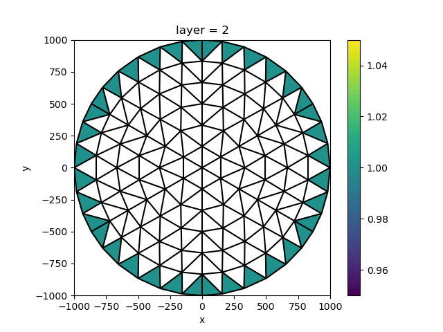
All the data above have been constants over the grid. For the constant head boundary, we’d like to only set values on the external border. We can py:method:xugrid.UgridDataset.binary_dilation to easily find these cells:

chd_location = xu.zeros_like(idomain.sel(layer=2), dtype=bool).ugrid.binary_dilation(
    border_value=True
)
constant_head = xu.full_like(idomain.sel(layer=2), 1.0, dtype=float).where(chd_location)

fig, ax = plt.subplots()
constant_head.ugrid.plot(ax=ax)
xu.plot.line(grid, ax=ax, color="black")
ax.set_aspect(1)

Write the model

The first step is to define an empty model, the parameters and boundary conditions are added in the form of the familiar MODFLOW packages.

gwf_model = imod.mf6.GroundwaterFlowModel()
gwf_model["disv"] = imod.mf6.VerticesDiscretization(
    top=10.0, bottom=bottom, idomain=idomain
)
gwf_model["chd"] = imod.mf6.ConstantHead(
    constant_head, print_input=True, print_flows=True, save_flows=True
)
gwf_model["ic"] = imod.mf6.InitialConditions(start=0.0)
gwf_model["npf"] = imod.mf6.NodePropertyFlow(
    icelltype=icelltype,
    k=k,
    k33=k33,
    save_flows=True,
)
gwf_model["sto"] = imod.mf6.SpecificStorage(
    specific_storage=1.0e-5,
    specific_yield=0.15,
    transient=False,
    convertible=0,
)
gwf_model["oc"] = imod.mf6.OutputControl(save_head="all", save_budget="all")
gwf_model["rch"] = imod.mf6.Recharge(rch_rate)

simulation = imod.mf6.Modflow6Simulation("circle")
simulation["GWF_1"] = gwf_model
simulation["solver"] = imod.mf6.Solution(
    modelnames=["GWF_1"],
    print_option="summary",
    outer_dvclose=1.0e-4,
    outer_maximum=500,
    under_relaxation=None,
    inner_dvclose=1.0e-4,
    inner_rclose=0.001,
    inner_maximum=100,
    linear_acceleration="cg",
    scaling_method=None,
    reordering_method=None,
    relaxation_factor=0.97,
)
simulation.create_time_discretization(additional_times=["2000-01-01", "2000-01-02"])

We’ll create a new directory in which we will write and run the model.

modeldir = imod.util.temporary_directory()
simulation.write(modeldir)

Run the model

Note

The following lines assume the mf6 executable is available on your PATH. The Modflow 6 examples introduction shortly describes how to add it to yours.

simulation.run()

Open the results

First, we’ll open the heads (.hds) file.

head = simulation.open_head()

head

<xarray.DataArray 'head' (time: 1, layer: 2, mesh2d_nFaces: 216)> Size: 3kB
dask.array<stack, shape=(1, 2, 216), dtype=float64, chunksize=(1, 2, 216), chunktype=numpy.ndarray>
Coordinates:
  * layer          (layer) int32 8B 1 2
  * time           (time) float64 8B 1.0
  * mesh2d_nFaces  (mesh2d_nFaces) int64 2kB 0 1 2 3 4 5 ... 211 212 213 214 215

xarray.DataArray

'head'

• time: 1
• layer: 2
• mesh2d_nFaces: 216

• dask.array<chunksize=(1, 2, 216), meta=np.ndarray>

  Array Chunk Bytes 3.38 kiB 3.38 kiB Shape (1, 2, 216) (1, 2, 216) Dask graph 1 chunks in 3 graph layers Data type float64 numpy.ndarray

• Coordinates: (3)
  • layer
    (layer)
    int32
    1 2

    array([1, 2])

  • time
    (time)
    float64
    1.0

    array([1.])

  • mesh2d_nFaces
    (mesh2d_nFaces)
    int64
    0 1 2 3 4 5 ... 211 212 213 214 215

    array([  0,   1,   2, ..., 213, 214, 215], dtype=int64)

• Indexes: (3)
  • layer
    PandasIndex

    PandasIndex(Index([1, 2], dtype='int32', name='layer'))

  • time
    PandasIndex

    PandasIndex(Index([1.0], dtype='float64', name='time'))

  • mesh2d_nFaces
    PandasIndex

    PandasIndex(RangeIndex(start=0, stop=216, step=1, name='mesh2d_nFaces'))

• Attributes: (0)

For a DISV MODFLOW6 model, the heads are returned as a UgridDataArray. While all layers are timesteps are available, they are only loaded into memory as needed.

We may also open the cell-by-cell flows (.cbc) file.

cbc = simulation.open_flow_budget()

print(cbc.keys())

KeysView(<xarray.Dataset> Size: 28kB
Dimensions:                 (layer: 2, time: 1, mesh2d_nEdges: 342,
                             mesh2d_nFaces: 216)
Coordinates:
  * layer                   (layer) int32 8B 1 2
  * time                    (time) float64 8B 1.0
  * mesh2d_nEdges           (mesh2d_nEdges) int64 3kB 0 1 2 3 ... 339 340 341
  * mesh2d_nFaces           (mesh2d_nFaces) int64 2kB 0 1 2 3 ... 213 214 215
Data variables:
    flow-horizontal-face    (time, layer, mesh2d_nEdges) float64 5kB dask.array<chunksize=(1, 2, 342), meta=np.ndarray>
    flow-horizontal-face-x  (time, layer, mesh2d_nEdges) float64 5kB dask.array<chunksize=(1, 2, 342), meta=np.ndarray>
    flow-horizontal-face-y  (time, layer, mesh2d_nEdges) float64 5kB dask.array<chunksize=(1, 2, 342), meta=np.ndarray>
    flow-lower-face         (time, layer, mesh2d_nFaces) float64 3kB dask.array<chunksize=(1, 2, 216), meta=np.ndarray>
    chd_chd                 (time, layer, mesh2d_nFaces) float64 3kB dask.array<chunksize=(1, 2, 216), meta=np.ndarray>)

The flows are returned as a dictionary of UgridDataArrays. This dictionary contains all entries that are stored in the CBC file, but like for the heads file the data are only loaded into memory when needed.

The horizontal flows are stored on the edges of the UgridDataArray topology. The other flows are generally stored on the faces; this includes the flow-lower-face.

We’ll create a dataset for the horizontal flows for further analysis.

cbc_grid = cbc["flow-horizontal-face-x"].grid
ds = xu.UgridDataset(grids=cbc_grid)
ds["u"] = cbc["flow-horizontal-face-x"]
ds["v"] = cbc["flow-horizontal-face-y"]

Visualize the results

We can quickly and easily visualize the output with the plotting functions provided by xarray and xugrid. We’ll add some some edge coordinates to the dataset so that they can be used to place the arrows in the quiver plot.

ds = ds.ugrid.assign_edge_coords()
fig, ax = plt.subplots()
head.isel(time=0, layer=0).compute().ugrid.plot(ax=ax)
ds.isel(time=0, layer=0).plot.quiver(
    x="mesh2d_edge_x", y="mesh2d_edge_y", u="u", v="v", color="white"
)
ax.set_aspect(1)

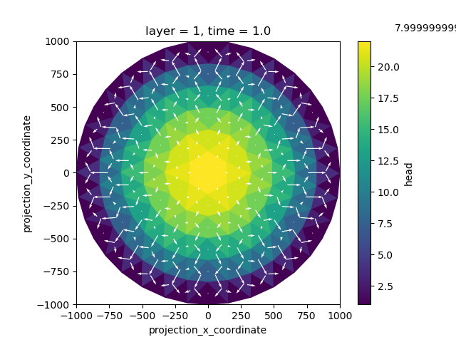
As would be expected from our model input, we observe circular groundwater mounding and increasing flows as we move from the center to the exterior.

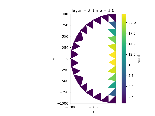
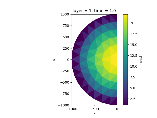
Slice the model domain

We may also quickly setup a smaller model. We’ll select half of the original domain. To set up the boundary conditions on the clipped edges you can provide a states_for_boundary dictionary. In this case we add the head values of the computed full domain simulation as the clipped boundary values

states_for_boundary = {
    "GWF_1": head.compute(),
}

half_simulation = simulation.clip_box(
    x_max=0.0, states_for_boundary=states_for_boundary
)

Let’s run the model, read the results, and visualize.

modeldir = imod.util.temporary_directory()
half_simulation.write(modeldir)
half_simulation.run()
head = half_simulation.open_head()

Let’s add constant head boundaries together and plot them

half_simulation_constant_head = half_simulation["GWF_1"]["chd"]["head"]

clipped_half_simulation_constant_head = (
    half_simulation["GWF_1"]["chd_clipped"]["head"].sel(layer=2).isel(time=0)
)

all_boundaries_constant_head = half_simulation_constant_head.where(
    ~isnull(half_simulation_constant_head), clipped_half_simulation_constant_head
)

# plot boundary conditions
fig, ax = plt.subplots()
all_boundaries_constant_head.ugrid.plot(ax=ax)
ax.set_aspect(1)

plot computed heads

fig, ax = plt.subplots()
head.isel(time=0, layer=0).compute().ugrid.plot(ax=ax)
ax.set_aspect(1)