Note
Go to the end to download the full example code.
Henry#
This example illustrates how to setup a variable density groundwater flow and
transport model using the imod package and associated packages.
In overview, we’ll set the following steps:
Create a suitable 2d (x, z) grid.
Create a groundwater flow model, with variable density.
Create a solute transport model.
Combine these models into a single MODFLOW 6 simulation.
Write to modflow6 files.
Run the model.
Open the results back into xarray DataArrays.
Visualize the results.
We are simulating the Henry problem, although not the original one but the one outlined in the MODFLOW 6 manual (jupyter notebooks example 51). This is the modified Henry problem with half the inflow rate.
The domain is a vertically oriented two dimensional rectangle, which is 2 m long and 1 m high. Water flows in over the left boundary with a fixed rate, which is represented by a Well package. The right boundary is in direct contact with hydrostatic seawater with a density of 1025 kg m:sup:-3. This is represented by a General Head Boundary package.
We’ll start with the usual imports. As this is a simple (synthetic) structured model, we can make do with few packages.
import numpy as np
import pandas as pd
import xarray as xr

import imod
We’ll start by defining the (vertical) rectangular domain and the physical parameters of the model.
nlay = 40
nrow = 1
ncol = 80
shape = (nlay, nrow, ncol)

total_flux = 5.7024  # m3/d
k = 864.0  # m/d
porosity = 0.35
max_concentration = 35.0
min_concentration = 0.0
max_density = 1025.0
min_density = 1000.0
diffusion_coefficient = 0.57024
longitudinal_horizontal = 0.1
transversal_horizontal1 = 0.01

# Time
start_date = pd.to_datetime("2020-01-01")
duration = pd.to_timedelta("0.5d")

# Domain size
xmax = 2.0
xmin = 0.0
dx = (xmax - xmin) / ncol
zmin = 0.0
zmax = 1.0
dz = (zmax - zmin) / nlay

x = np.arange(xmin, xmax, dx) + 0.5 * dx
y = np.array([0.5])
layer = np.arange(1, 41, 1)

dy = -1.0
coords = {"layer": layer, "y": y, "x": x, "dy": dy, "dx": dx}
dims = ("layer", "y", "x")
idomain = xr.DataArray(np.ones(shape, dtype=int), coords=coords, dims=dims)

top = 1.0
bottom = xr.DataArray(
    np.arange(zmin, zmax, dz)[::-1],
    {"layer": layer},
    ("layer",),
)
Now make the flow model. We’ll start with the non-boundary condition packages.
gwf_model = imod.mf6.GroundwaterFlowModel()
gwf_model["dis"] = imod.mf6.StructuredDiscretization(
    top=top, bottom=bottom, idomain=idomain
)
gwf_model["npf"] = imod.mf6.NodePropertyFlow(
    icelltype=0,
    k=k,
)
gwf_model["sto"] = imod.mf6.SpecificStorage(
    specific_storage=1.0e-4,
    specific_yield=0.15,
    transient=False,
    convertible=0,
)
gwf_model["ic"] = imod.mf6.InitialConditions(start=0.0)
gwf_model["oc"] = imod.mf6.OutputControl(save_head="last", save_budget="last")
Now let’s make the constant head boundary condition.
ghb_head = xr.ones_like(idomain, dtype=float)
ghb_head[:, :, :-1] = np.nan

ghb_conc = xr.full_like(idomain, max_concentration, dtype=float)
ghb_conc[:, :, :-1] = np.nan
ghb_conc = ghb_conc.expand_dims(species=["salinity"])

conductance = xr.full_like(idomain, 864.0 * 2.0, dtype=float)
conductance[:, :, :-1] = np.nan

gwf_model["right_boundary"] = imod.mf6.GeneralHeadBoundary(
    head=ghb_head,
    conductance=conductance,
    concentration=ghb_conc,
    concentration_boundary_type="AUX",
    print_input=True,
    print_flows=True,
    save_flows=True,
)
… and the constant flux condition.
from imod.prepare import create_layered_top

screen_top = create_layered_top(bottom, top)

flux_concentration = xr.DataArray(
    data=np.full((1, nlay), min_concentration),
    dims=["species", "index"],
    coords={"species": ["salinity"], "index": layer},
)

gwf_model["left_boundary"] = imod.mf6.Well(
    x=np.full_like(layer, xmin, dtype=float),
    y=np.full_like(layer, y[0], dtype=float),
    screen_top=screen_top.values,
    screen_bottom=bottom.values,
    rate=np.full_like(layer, 0.5 * (total_flux / nlay), dtype=float),
    concentration=flux_concentration,
    concentration_boundary_type="AUX",
    minimum_thickness=0.002,
)
Since we are solving a variable density problem, we need to add the buoyancy package. It will use the species “salinity” that we are simulating with a transport model defined below.
slope = (max_density - min_density) / (max_concentration - min_concentration)
gwf_model["buoyancy"] = imod.mf6.Buoyancy(
    reference_density=min_density,
    modelname=["transport"],
    reference_concentration=[min_concentration],
    density_concentration_slope=[slope],
    species=["salinity"],
)
Now let’s make the transport model. It contains the standard packages of storage, dispersion and advection as well as initial condiations and output control. Sinks and sources are automatically determined based on packages provided in the flow model.
gwt_model = imod.mf6.GroundwaterTransportModel()
gwt_model["ssm"] = imod.mf6.SourceSinkMixing.from_flow_model(gwf_model, "salinity")
gwt_model["adv"] = imod.mf6.AdvectionTVD()
gwt_model["dsp"] = imod.mf6.Dispersion(
    diffusion_coefficient=0.57024,
    longitudinal_horizontal=0.1,
    transversal_horizontal1=0.01,
    xt3d_off=False,
    xt3d_rhs=False,
)

gwt_model["mst"] = imod.mf6.MobileStorageTransfer(
    porosity=porosity,
)
gwt_model["ic"] = imod.mf6.InitialConditions(start=max_concentration)
gwt_model["oc"] = imod.mf6.OutputControl(save_concentration="last", save_budget="last")
gwt_model["dis"] = gwf_model["dis"]
Now let’s define a simulation using the flow and transport models.
# Attach it to a simulation
simulation = imod.mf6.Modflow6Simulation("henry")

simulation["flow"] = gwf_model
simulation["transport"] = gwt_model
Define solver settings. We need to define separate solutions for the flow and transport models. In this case, we’ll use the same settings, but generally convergence settings should differ: the transport model has very different units from the flow model.
simulation["flow_solver"] = imod.mf6.Solution(
    modelnames=["flow"],
    print_option="summary",
    outer_dvclose=1.0e-6,
    outer_maximum=500,
    under_relaxation=None,
    inner_dvclose=1.0e-6,
    inner_rclose=1.0e-10,
    inner_maximum=100,
    linear_acceleration="bicgstab",
    scaling_method=None,
    reordering_method=None,
    relaxation_factor=0.97,
)
simulation["transport_solver"] = imod.mf6.Solution(
    modelnames=["transport"],
    print_option="summary",
    outer_dvclose=1.0e-6,
    outer_maximum=500,
    under_relaxation=None,
    inner_dvclose=1.0e-6,
    inner_rclose=1.0e-10,
    inner_maximum=100,
    linear_acceleration="bicgstab",
    scaling_method=None,
    reordering_method=None,
    relaxation_factor=0.97,
)
# Collect time discretization
times = [start_date, start_date + duration]
simulation.create_time_discretization(additional_times=times)
Increase the number of time steps for the single stress period:
simulation["time_discretization"]["n_timesteps"] = 500
We’ll create a new directory in which we will write and run the model.
modeldir = imod.util.temporary_directory()
simulation.write(modeldir, binary=False)
Run the model#
This takes about 20 seconds.
Note
The following lines assume the mf6 executable is available on your PATH.
The MODFLOW 6 examples introduction shortly
describes how to add it to yours.
simulation.run()
Open the results#
We’ll open the head and concentration files.
head = simulation.open_head()

conc = simulation.open_concentration()
Visualize the results#
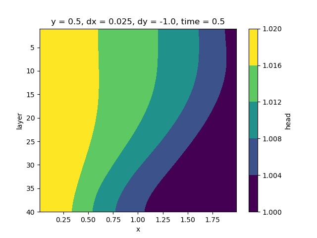
head.isel(y=0, time=-1).plot.contourf(yincrease=False)

<matplotlib.contour.QuadContourSet object at 0x0000019B35889220>
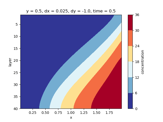
We can check the concentration to see that a fresh-saline interface has been formed:
conc.isel(y=0, time=-1).plot.contourf(yincrease=False, cmap="RdYlBu_r")

<matplotlib.contour.QuadContourSet object at 0x0000019B2DC402F0>
Total running time of the script: (0 minutes 39.794 seconds)