TWRI

This example has been converted from the MODFLOW6 Example problems. See the description and the notebook which uses FloPy to setup the model.

This example is a modified version of the original MODFLOW example (”Techniques of Water-Resources Investigation” (TWRI)) described in (McDonald & Harbaugh, 1988) and duplicated in (Harbaugh & McDonald, 1996). This problem is also is distributed with MODFLOW-2005 (Harbaugh, 2005). The problem has been modified from a quasi-3D problem, where confining beds are not explicitly simulated, to an equivalent three-dimensional problem.

In overview, we’ll set the following steps:

• Create a structured grid for a rectangular geometry.

• Create the xarray DataArrays containg the MODFLOW6 parameters.

• Feed these arrays into the imod mf6 classes.

• Write to modflow6 files.

• Run the model.

• Open the results back into DataArrays.

• Visualize the results.

We’ll start with the usual imports. As this is an simple (synthetic) structured model, we can make due with few packages.

import numpy as np
import xarray as xr

import imod

Create grid coordinates

The first steps consist of setting up the grid – first the number of layer, rows, and columns. Cell sizes are constant throughout the model.

nlay = 3
nrow = 15
ncol = 15
shape = (nlay, nrow, ncol)

dx = 5000.0
dy = -5000.0
xmin = 0.0
xmax = dx * ncol
ymin = 0.0
ymax = abs(dy) * nrow
dims = ("layer", "y", "x")

layer = np.array([1, 2, 3])
y = np.arange(ymax, ymin, dy) + 0.5 * dy
x = np.arange(xmin, xmax, dx) + 0.5 * dx
coords = {"layer": layer, "y": y, "x": x}

Create DataArrays

Now that we have the grid coordinates setup, we can start defining model parameters. The model is characterized by:

• a constant head boundary on the left

• a single drain in the center left of the model

• uniform recharge on the top layer

• a number of wells scattered throughout the model.

idomain = xr.DataArray(np.ones(shape, dtype=int), coords=coords, dims=dims)
bottom = xr.DataArray([-200.0, -300.0, -450.0], {"layer": layer}, ("layer",))

# Constant head
constant_head = xr.full_like(idomain, np.nan, dtype=float).sel(layer=[1, 2])
constant_head[..., 0] = 0.0

# Drainage
elevation = xr.full_like(idomain.sel(layer=1), np.nan, dtype=float)
conductance = xr.full_like(idomain.sel(layer=1), np.nan, dtype=float)
elevation[7, 1:10] = np.array([0.0, 0.0, 10.0, 20.0, 30.0, 50.0, 70.0, 90.0, 100.0])
conductance[7, 1:10] = 1.0

# Recharge
rch_rate = xr.full_like(idomain.sel(layer=1), 3.0e-8, dtype=float)

# Well
# fmt: off
wells_x = [52500.0, 27500.0, 57500.0, 37500.0, 47500.0, 57500.0, 67500.0, 37500.0,
           47500.0, 57500.0, 67500.0, 37500.0, 47500.0, 57500.0, 67500.0, ]
wells_y = [52500.0, 57500.0, 47500.0, 32500.0, 32500.0, 32500.0, 32500.0, 22500.0,
           22500.0, 22500.0, 22500.0, 12500.0, 12500.0, 12500.0, 12500.0, ]
screen_top = [-300.0, -200.0, -200.0, 200.0, 200.0, 200.0, 200.0, 200.0,
              200.0, 200.0, 200.0, 200.0, 200.0, 200.0, 200.0, ]
screen_bottom = [-450.0, -300.0, -300.0, -200.0, -200.0, -200.0, -200.0, -200.0,
                 -200.0, -200.0, -200.0, -200.0, -200.0, -200.0, -200.0, ]
rate_wel = [-5.0, -5.0, -5.0, -5.0, -5.0, -5.0, -5.0, -5.0,
            -5.0, -5.0, -5.0, -5.0, -5.0, -5.0, -5.0, ]
# fmt: on

# Node properties
icelltype = xr.DataArray([1, 0, 0], {"layer": layer}, ("layer",))
k = xr.DataArray([1.0e-3, 1.0e-4, 2.0e-4], {"layer": layer}, ("layer",))
k33 = xr.DataArray([2.0e-8, 2.0e-8, 2.0e-8], {"layer": layer}, ("layer",))

Write the model

The first step is to define an empty model, the parameters and boundary conditions are added in the form of the familiar MODFLOW packages.

gwf_model = imod.mf6.GroundwaterFlowModel()
gwf_model["dis"] = imod.mf6.StructuredDiscretization(
    top=200.0, bottom=bottom, idomain=idomain
)
gwf_model["chd"] = imod.mf6.ConstantHead(
    constant_head, print_input=True, print_flows=True, save_flows=True
)
gwf_model["drn"] = imod.mf6.Drainage(
    elevation=elevation,
    conductance=conductance,
    print_input=True,
    print_flows=True,
    save_flows=True,
)
gwf_model["ic"] = imod.mf6.InitialConditions(start=0.0)
gwf_model["npf"] = imod.mf6.NodePropertyFlow(
    icelltype=icelltype,
    k=k,
    k33=k33,
    variable_vertical_conductance=True,
    dewatered=True,
    perched=True,
    save_flows=True,
)
gwf_model["sto"] = imod.mf6.SpecificStorage(
    specific_storage=1.0e-5,
    specific_yield=0.15,
    transient=False,
    convertible=0,
)
gwf_model["oc"] = imod.mf6.OutputControl(save_head="all", save_budget="all")
gwf_model["rch"] = imod.mf6.Recharge(rch_rate)

gwf_model["wel"] = imod.mf6.Well(
    x=wells_x,
    y=wells_y,
    screen_top=screen_top,
    screen_bottom=screen_bottom,
    rate=rate_wel,
    minimum_k=0.0001,
)

# Attach it to a simulation
simulation = imod.mf6.Modflow6Simulation("ex01-twri")
simulation["GWF_1"] = gwf_model
# Define solver settings
simulation["solver"] = imod.mf6.Solution(
    modelnames=["GWF_1"],
    print_option="summary",
    outer_dvclose=1.0e-4,
    outer_maximum=500,
    under_relaxation=None,
    inner_dvclose=1.0e-4,
    inner_rclose=0.001,
    inner_maximum=100,
    linear_acceleration="cg",
    scaling_method=None,
    reordering_method=None,
    relaxation_factor=0.97,
)
# Collect time discretization
simulation.create_time_discretization(
    additional_times=["2000-01-01", "2000-01-02", "2000-01-03", "2000-01-04"]
)

We’ll create a new directory in which we will write and run the model.

modeldir = imod.util.temporary_directory()
simulation.write(modeldir)

Run the model

Note

The following lines assume the mf6 executable is available on your PATH. The Modflow 6 examples introduction shortly describes how to add it to yours.

simulation.run()

Open the results

We’ll open the heads (.hds) file.

head = imod.mf6.open_hds(
    modeldir / "GWF_1/GWF_1.hds",
    modeldir / "GWF_1/dis.dis.grb",
)

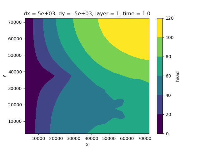
Visualize the results

head.isel(layer=0, time=0).plot.contourf()

<matplotlib.contour.QuadContourSet object at 0x00000204CEFB4710>