Note
Go to the end to download the full example code.
Transport 2d example#
The simulation shown here comes from the 1999 MT3DMS report, p 138: Two-Dimensional Transport in a Uniform Flow of solute injected continuously from a point source in a steady-state uniform flow field.
In this example, we build up the model, and the we run the model as is. Next, we split the model in 4 partitions and run that as well. Finally, we show that the difference in outcome for the partitioned and unpartitioned models is small.
MT3DMS: A Modular Three-Dimensional Multispecies Transport Model for Simulation of Advection, Dispersion, and Chemical Reactions of Contaminants in Groundwater Systems; Documentation and User’s Guide
import matplotlib.pyplot as plt
import numpy as np
import pandas as pd
import xarray as xr

import imod
from imod.typing.grid import nan_like, zeros_like
Set some grid dimensions
nlay = 1  # Number of layers
nrow = 31  # Number of rows
ncol = 46  # Number of columns
delr = 10.0  # Column width ($m$)
delc = 10.0  # Row width ($m$)
delz = 10.0  # Layer thickness ($m$)
shape = (nlay, nrow, ncol)
top = 10.0
dims = ("layer", "y", "x")
Construct the “idomain” array, and then the discretization package which represents the model grid.
y = np.arange(delr * nrow, 0, -delr)
x = np.arange(0, delc * ncol, delc)
coords = {"layer": [1], "y": y, "x": x, "dx": delc, "dy": -delr}
idomain = xr.DataArray(np.ones(shape, dtype=int), coords=coords, dims=dims)

bottom = xr.DataArray([0.0], {"layer": [1]}, ("layer",))
gwf_model = imod.mf6.GroundwaterFlowModel()
gwf_model["dis"] = imod.mf6.StructuredDiscretization(
    top=10.0, bottom=bottom, idomain=idomain
)
Construct the other flow packages. Flow is steady-state in this simulation, meaning specific storage is set to zero.
gwf_model["sto"] = imod.mf6.SpecificStorage(
    specific_storage=0.0,
    specific_yield=0.0,
    transient=False,
    convertible=0,
)
gwf_model["npf"] = imod.mf6.NodePropertyFlow(
    icelltype=zeros_like(idomain), k=1.0, save_flows=True, save_specific_discharge=True
)
gwf_model["oc"] = imod.mf6.OutputControl(save_head="all", save_budget="all")
gwf_model["ic"] = imod.mf6.InitialConditions(start=10.0)
Set up the boundary conditions. We have: 2 constant head boundaries at the left and right, chosen so that the velocity is 1/3 m/day and a well that injects 1 m3 per day, with a concentration of 1000
Lx = 460
v = 1.0 / 3.0
prsity = 0.3
q = v * prsity
h1 = q * Lx
chd_field = nan_like(idomain)
chd_field.values[0, :, 0] = h1
chd_field.values[0, :, -1] = 0.0
chd_concentration = nan_like(idomain)
chd_concentration.values[0, :, 0] = 0.0
chd_concentration.values[0, :, -1] = 0.0
chd_concentration = chd_concentration.expand_dims(species=["Au"])


gwf_model["chd"] = imod.mf6.ConstantHead(
    chd_field,
    concentration=chd_concentration,
    print_input=True,
    print_flows=True,
    save_flows=True,
)
injection_concentration = xr.DataArray(
    [[1000.0]],
    coords={
        "species": ["Au"],
        "index": [0],
    },
    dims=("species", "index"),
)
gwf_model["wel"] = imod.mf6.Well(
    x=[150.0],
    y=[150.0],
    screen_top=[10.0],
    screen_bottom=[0.0],
    rate=[1.0],
    concentration=injection_concentration,
    concentration_boundary_type="aux",
)
Now construct the transport simulation. The flow boundaries already have inflow concentration data associated, so the transport boundaries can be imported using the ssm package, and the rest of the transport model definition is straightforward.
tpt_model = imod.mf6.GroundwaterTransportModel()
tpt_model["ssm"] = imod.mf6.SourceSinkMixing.from_flow_model(
    gwf_model, species="Au", save_flows=True
)
tpt_model["adv"] = imod.mf6.AdvectionUpstream()
tpt_model["dsp"] = imod.mf6.Dispersion(
    diffusion_coefficient=0.0,
    longitudinal_horizontal=10.0,
    transversal_horizontal1=3.0,
    xt3d_off=False,
    xt3d_rhs=False,
)
tpt_model["mst"] = imod.mf6.MobileStorageTransfer(
    porosity=0.3,
)

tpt_model["ic"] = imod.mf6.InitialConditions(start=0.0)
tpt_model["oc"] = imod.mf6.OutputControl(save_concentration="all", save_budget="last")
tpt_model["dis"] = gwf_model["dis"]
Create a simulation and add the flow and transport models to it. Then define some ims packages: 1 for every type of model. Finally create 365 time steps of 1 day each.
simulation = imod.mf6.Modflow6Simulation("ex01-twri")
simulation["GWF_1"] = gwf_model
simulation["TPT_1"] = tpt_model


simulation["flow_solver"] = imod.mf6.Solution(
    modelnames=["GWF_1"],
    print_option="summary",
    outer_dvclose=1.0e-4,
    outer_maximum=500,
    under_relaxation=None,
    inner_dvclose=1.0e-4,
    inner_rclose=0.001,
    inner_maximum=100,
    linear_acceleration="cg",
    scaling_method=None,
    reordering_method=None,
    relaxation_factor=0.97,
)
simulation["transport_solver"] = imod.mf6.Solution(
    modelnames=["TPT_1"],
    print_option="summary",
    outer_dvclose=1.0e-4,
    outer_maximum=500,
    under_relaxation=None,
    inner_dvclose=1.0e-4,
    inner_rclose=0.001,
    inner_maximum=100,
    linear_acceleration="bicgstab",
    scaling_method=None,
    reordering_method=None,
    relaxation_factor=0.97,
)
# Collect time discretization

duration = pd.to_timedelta("365d")
start = pd.to_datetime("2002-01-01")
simulation.create_time_discretization(additional_times=[start, start + duration])
simulation["time_discretization"]["n_timesteps"] = 365
modeldir = imod.util.temporary_directory()
simulation.write(modeldir, binary=False)
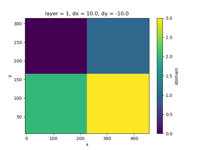
To split the model in 4 partitions, we must create a label array.
We use the utility function get_label_array for that.
label_array = simulation.create_partition_labels(4)
fig, ax = plt.subplots()
label_array.plot(ax=ax)
<matplotlib.collections.QuadMesh object at 0x0000019B2F1580B0>
This label array determines how the model will be split. METIS is used in the background to partition models, which is the cause of the imperfect rectangular shapes. Let’s split the simulation into 4 submodels. The label array is used to define the partitioning.
split_simulation = simulation.split(label_array)
C:\buildagent\work\4b9080cbb3354582\imod-python\.pixi\envs\default\Lib\site-packages\xarray\core\duck_array_ops.py:250: RuntimeWarning: invalid value encountered in cast
  return data.astype(dtype, **kwargs)
C:\buildagent\work\4b9080cbb3354582\imod-python\.pixi\envs\default\Lib\site-packages\xarray\core\duck_array_ops.py:250: RuntimeWarning: invalid value encountered in cast
  return data.astype(dtype, **kwargs)
C:\buildagent\work\4b9080cbb3354582\imod-python\.pixi\envs\default\Lib\site-packages\xarray\core\duck_array_ops.py:250: RuntimeWarning: invalid value encountered in cast
  return data.astype(dtype, **kwargs)
C:\buildagent\work\4b9080cbb3354582\imod-python\.pixi\envs\default\Lib\site-packages\xarray\core\duck_array_ops.py:250: RuntimeWarning: invalid value encountered in cast
  return data.astype(dtype, **kwargs)
Run the unsplit model and load the simulation results.
simulation.run()
conc = simulation.open_concentration()
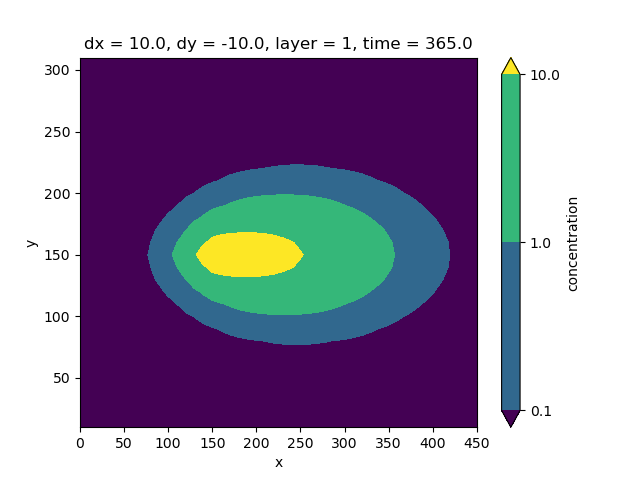
Run the split model and load the simulation results.
split_modeldir = modeldir / "split"
split_simulation.write(split_modeldir, binary=False)
split_simulation.run()
split_conc = split_simulation.open_concentration()["concentration"]
fig, ax = plt.subplots()
split_conc.isel(layer=0, time=364).plot.contourf(ax=ax, levels=[0.1, 1, 10])
<matplotlib.contour.QuadContourSet object at 0x0000019B358226C0>
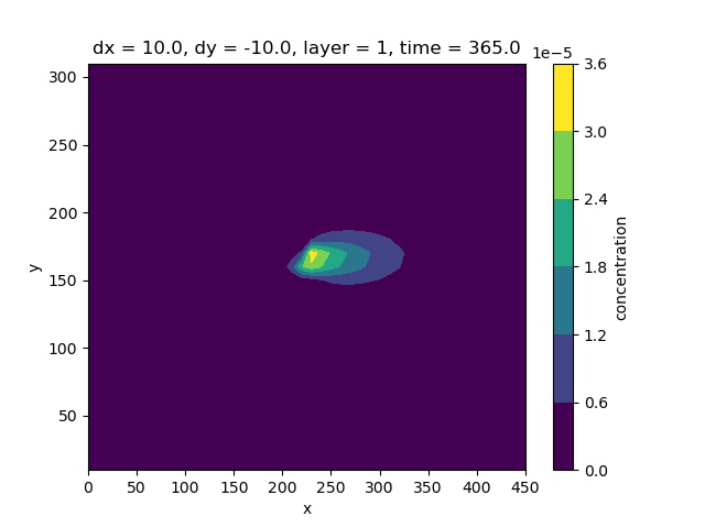
Compute the difference between the split and unsplit simulation results for transport at the end of the simulation, and print them
diff = abs(conc - split_conc)
fig, ax = plt.subplots()
diff.isel(layer=0, time=364).plot.contourf(ax=ax)
<matplotlib.contour.QuadContourSet object at 0x0000019B358A68A0>
Total running time of the script: (0 minutes 57.121 seconds)