Note
Go to the end to download the full example code.
Freshwater lens (circle)#
This example illustrates how to setup a very simple unstructured groundwater
transport model using the imod package and associated packages.
In overview, we’ll set the following steps:
Setting up the flow model, just like in the Circle example
set up the transport model
Run the simulation.
Visualize the results.
We’ll start with the following imports:
import matplotlib.pyplot as plt
import numpy as np
import pandas as pd
import xarray as xr
import xugrid as xu

import imod
Parameters#
porosity = 0.10
max_concentration = 35.0
min_concentration = 0.0
max_density = 1025.0
min_density = 1000.0
k_value = 10.0
Create a mesh#
The first steps consists of generating a mesh. In this example, we’ll use data included with iMOD Python for a circular mesh. Note that this is a Ugrid2D object. For more information on working with unstructured grids see the Xugrid documentation
grid_triangles = imod.data.circle()

fig, ax = plt.subplots()
xu.plot.line(grid_triangles)
ax.set_aspect(1)
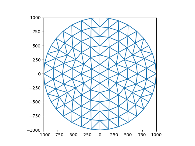
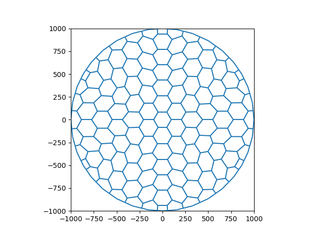
However a triangular grid has the issue that the direction of the fluxes between cell centres is not perpendicular to the cell vertices. The default formulation of MODFLOW 6 does not account for this, which causes mass balance errors. The XT3D formulation is able to account for this, but the last version of MODFLOW 6 (6.3 at time of writing) does not support this in combination with the Buoyancy package and using XT3D comes with an extra, significant computational burden. It is therefore easier to use a voronoi grid, for which Xugrid has a very convenient method.
grid = grid_triangles.tesselate_centroidal_voronoi()

fig, ax = plt.subplots()
xu.plot.line(grid)
ax.set_aspect(1)
Create arrays
nface = grid.n_face
nlayer = 15

layer = np.arange(nlayer, dtype=int) + 1

idomain = xu.UgridDataArray(
    xr.DataArray(
        np.ones((nlayer, nface), dtype=np.int32),
        coords={"layer": layer},
        dims=["layer", grid.face_dimension],
    ),
    grid=grid,
)
icelltype = xu.full_like(idomain, 0)
k = xu.full_like(idomain, k_value, dtype=float)
k33 = k.copy()

top = 0.0
bottom = xr.DataArray(top - (layer * 10.0), dims=["layer"])
Recharge#
We need a recharge rate for the fluid and a recharge rate for the solute. The fluid recharge rate is volumetric and per unit area, so the unit is length/time. The solute recharge rate is the concentration of solute in the recharge, and has concentration units.
rch_rate = xu.full_like(idomain.sel(layer=1), 0.001, dtype=float)
rch_concentration = xu.full_like(rch_rate, min_concentration)
rch_concentration = rch_concentration.expand_dims(species=["salinity"])
Unlike a recharge boundary, with a prescribed head boundary we don’t know a priori whether water will flow in over the boundary or leave across the boundary. If water flows into the model over the boundary, it carries a prescribed solute concentration. If it leaves, it leaves with the concentration that was computed for the cell.
In this example we set the prescribed head value to 0.0 and the external concentration to 35.0 as well. The boundary only operates on the top layer.
ghb_location = xu.zeros_like(idomain.sel(layer=1), dtype=bool).ugrid.binary_dilation(
    border_value=True
)
constant_head = xu.full_like(idomain, 0.0, dtype=float).where(ghb_location)
conductance = (idomain * grid.area * k_value).where(ghb_location)

constant_concentration = xu.full_like(constant_head, max_concentration).where(
    ghb_location
)
constant_concentration = constant_concentration.expand_dims(species=["salinity"])
Add flow model to simulation#
See the Circle example for more information.
gwf_model = imod.mf6.GroundwaterFlowModel()
gwf_model["disv"] = imod.mf6.VerticesDiscretization(
    top=top, bottom=bottom, idomain=idomain
)
gwf_model["ghb"] = imod.mf6.GeneralHeadBoundary(
    constant_head,
    conductance=conductance,
    concentration=constant_concentration,
    print_input=True,
    print_flows=True,
    save_flows=True,
)
gwf_model["ic"] = imod.mf6.InitialConditions(start=0.0)
gwf_model["npf"] = imod.mf6.NodePropertyFlow(
    icelltype=icelltype,
    k=k,
    k33=k33,
    save_flows=True,
)
gwf_model["sto"] = imod.mf6.SpecificStorage(
    specific_storage=1.0e-5,
    specific_yield=0.15,
    transient=False,
    convertible=0,
)
gwf_model["oc"] = imod.mf6.OutputControl(save_head="last", save_budget="last")
gwf_model["rch"] = imod.mf6.Recharge(
    rch_rate, concentration=rch_concentration, print_flows=True, save_flows=True
)

simulation = imod.mf6.Modflow6Simulation("circle")
simulation["flow"] = gwf_model
simulation["flow_solver"] = imod.mf6.Solution(
    modelnames=["flow"],
    print_option="summary",
    outer_dvclose=1.0e-4,
    outer_maximum=500,
    under_relaxation=None,
    inner_dvclose=1.0e-4,
    inner_rclose=0.001,
    inner_maximum=100,
    linear_acceleration="bicgstab",
    scaling_method=None,
    reordering_method=None,
    relaxation_factor=0.97,
)
Time discretization#
Set the timesteps, we want output each year, so we specify stress periods which last 1 year. We add the additional times to ensure that there is output at the end of each year. To achieve this we setup stress periods were each stress period is a year long. We can then use the “last” keyword in the output control to save the output.
simtimes = pd.date_range(start="2000-01-01", end="2030-01-01", freq="As")
simulation.create_time_discretization(additional_times=simtimes)
We want to use adaptive time stepping to ensure stable results without taking
an unnecessary amount of small timesteps. We set the initial time step to 0.1
day, the minimum time step to 0.1 day, and the maximum time step to 50 days.
The multiplier is set to 2.0 so that consecutive timesteps will be increased
by a factor of 2 if the convergence is good. Furthermore, we will set the
ats_percel to 0.95 in the Advection package in the next section to let
MODFLOW 6 compute an appropriate time step based on the velocity field: A
solute parcel should not travel more than one cell in a time step. From these
two criteria MODFLOW 6 will select the smallest time step.
simulation["ats"] = imod.mf6.AdaptiveTimeStepping(
    dt_init=1e-1,
    dt_min=1e-1,
    dt_max=50.0,
    dt_multiplier=2.0,
)
Buoyancy#
Since we are solving a variable density problem, we need to add the buoyancy package. It will use the species “salinity” that we are simulating with a transport model defined below.
slope = (max_density - min_density) / (max_concentration - min_concentration)
gwf_model["buoyancy"] = imod.mf6.Buoyancy(
    reference_density=min_density,
    modelname=["transport"],
    reference_concentration=[min_concentration],
    density_concentration_slope=[slope],
    species=["salinity"],
)
Add transport model to simulation#
The transport model requires the flow field inside the domain computed by the flow model. It also needs the fluxes over the boundary. It uses the same discretization as the flow model. Here we create a transport model for salinity, derive sources and sinks based from the flow model, and tell it to use the same discretization.
transport_model = imod.mf6.GroundwaterTransportModel()
transport_model["ssm"] = imod.mf6.SourceSinkMixing.from_flow_model(
    gwf_model, "salinity"
)
transport_model["disv"] = gwf_model["disv"]
Now we define some transport packages for simulating the physical processes of advection, mechanical dispersion, and molecular diffusion dispersion. This example is transient, and the volume available for storage is the porosity, in this case 0.10.
al = 0.001

transport_model["dsp"] = imod.mf6.Dispersion(
    diffusion_coefficient=1e-4,
    longitudinal_horizontal=al,
    transversal_horizontal1=al * 0.1,
    transversal_vertical=al * 0.01,
    xt3d_off=False,
    xt3d_rhs=False,
)
transport_model["adv"] = imod.mf6.AdvectionTVD(ats_percel=0.95)
transport_model["mst"] = imod.mf6.MobileStorageTransfer(porosity)
Define the maximum concentration as the initial conditions, also output options for the transport model, and assign the transport model to the simulation as well.
transport_model["ic"] = imod.mf6.InitialConditions(start=max_concentration)
transport_model["oc"] = imod.mf6.OutputControl(
    save_concentration="last", save_budget="last"
)

simulation["transport"] = transport_model
simulation["transport_solver"] = imod.mf6.Solution(
    modelnames=["transport"],
    print_option="summary",
    outer_dvclose=1.0e-4,
    outer_maximum=500,
    under_relaxation=None,
    inner_dvclose=1.0e-4,
    inner_rclose=0.001,
    inner_maximum=100,
    linear_acceleration="bicgstab",
    scaling_method=None,
    reordering_method=None,
    relaxation_factor=0.97,
)
We’ll create a new directory in which we will write and run the model.
modeldir = imod.util.temporary_directory() / "full"
simulation.write(modeldir, binary=False)
Run the model#
Note
The following lines assume the mf6 executable is available on your
PATH. The examples introduction shortly describes how to add it to yours.
simulation.run()
Open the results#
sim_concentration = simulation.open_concentration().compute().reindex_like(idomain)
sim_head = simulation.open_head().compute().reindex_like(idomain)
Assign coordinates to output#
The model output does not feature very useful coordinate values for time
and z, therefore it is best to assign these to the datasets for more
understandable plots.
First we have to compute values for a z coordinate. The
interfaces = np.concatenate([[top], bottom.values])
z = (interfaces[:-1] + interfaces[1:]) / 2

z
array([  -5.,  -15.,  -25.,  -35.,  -45.,  -55.,  -65.,  -75.,  -85.,
        -95., -105., -115., -125., -135., -145.])
Assign these new coordinate values to the dataset
coords = {"time": simtimes[1:], "z": ("layer", z)}

sim_head = sim_head.assign_coords(**coords)
sim_concentration = sim_concentration.assign_coords(**coords)
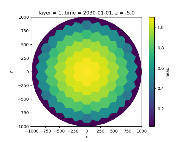
Visualize the results#
We can quickly and easily visualize the output with the plotting functions provided by xarray and xugrid:
fig, ax = plt.subplots()
sim_head.isel(time=-1, layer=0).ugrid.plot(ax=ax)
ax.set_aspect(1)
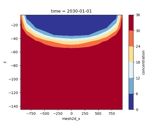
We can draw a crossection through the center by selecting y=0, for which we can plot the contours as follows:
fig, ax = plt.subplots()
sim_concentration.isel(time=-1).ugrid.sel(y=0).plot.contourf(
    ax=ax, x="mesh2d_x", y="z", cmap="RdYlBu_r"
)
<matplotlib.contour.QuadContourSet object at 0x0000019B382068A0>
Slice the model domain#
We may also quickly setup a smaller model. We’ll select half of the original domain. To set up the boundary conditions on the clipped edges you can provide a states_for_boundary dictionary. In this case we add the head values for the flow model and the concentration values for the transport model of the computed full domain simulation as the clipped boundary values. You can use this feature to clip a smaller model from an existing larger model, downscale it, and conduct a study in more detail around an area of interest.
states_for_boundary = {
    "flow": sim_head.isel(time=-1, drop=True).drop_vars("z"),
    "transport": sim_concentration.isel(time=-1, drop=True).drop_vars("z"),
}

half_simulation = simulation.clip_box(
    x_max=0.1, states_for_boundary=states_for_boundary
)
Let’s run the model, read the results, and visualize.
modeldir = imod.util.temporary_directory() / "half"
half_simulation.write(modeldir)
half_simulation.run()
Open the results#
half_sim_concentration = half_simulation.open_concentration().compute()
half_sim_head = half_simulation.open_head().compute()
Assign these new coordinate values to the dataset
half_sim_head = half_sim_head.assign_coords(**coords)
half_sim_concentration = half_sim_concentration.assign_coords(**coords)
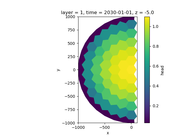
Visualize the results#
We can quickly and easily visualize the output with the plotting functions provided by xarray and xugrid:
fig, ax = plt.subplots()
half_sim_head.isel(time=-1, layer=0).ugrid.plot(ax=ax)
ax.set_aspect(1)
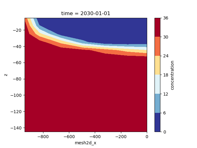
We can draw a crossection through the center by selecting y=0, for which we can plot the contours as follows:
fig, ax = plt.subplots()
half_sim_concentration.isel(time=-1).ugrid.sel(y=0).plot.contourf(
    ax=ax, x="mesh2d_x", y="z", cmap="RdYlBu_r"
)
<matplotlib.contour.QuadContourSet object at 0x0000019B381E5D60>
Total running time of the script: (1 minutes 16.796 seconds)