Note
Go to the end to download the full example code.
Regridding overview#
Regridding is the process of converting gridded data from one grid to another grid. Xugrid provides tools for 2D and 3D regridding of structured gridded data, represented as xarray objects, as well as (layered) unstructured gridded data, represented as xugrid objects.
A number of regridding methods are provided, based on area or volume overlap, as well as interpolation routines. It currently only supports Cartesian coordinates. See e.g. xESMF instead for regridding with a spherical Earth representation (note: EMSF is not available via conda-forge on Windows).
Here are a number of quick examples of how to get started with regridding.
We’ll start by importing a few essential packages.
import matplotlib.pyplot as plt
import xarray as xr

import xugrid as xu
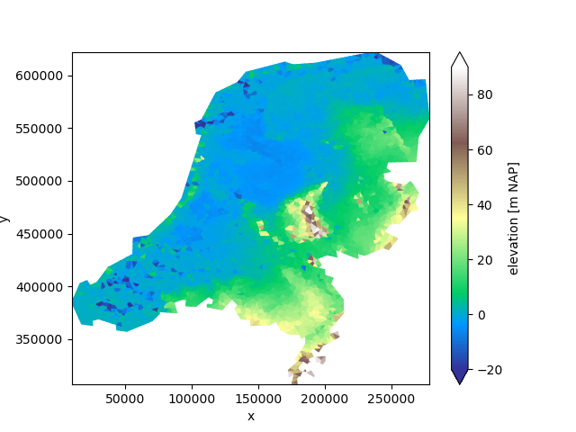
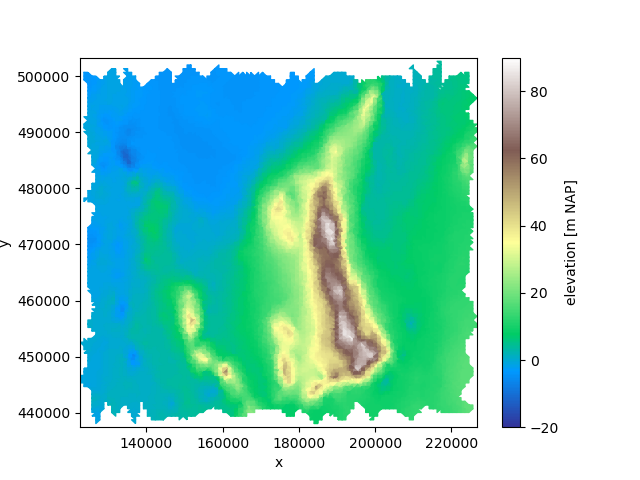
We will take a look at a sample dataset: a triangular grid with the surface elevation of the Netherlands.
uda = xu.data.elevation_nl()
uda.ugrid.plot(vmin=-20, vmax=90, cmap="terrain")
<matplotlib.collections.PolyCollection object at 0x7feaafa1e360>
Xugrid provides several “regridder” classes which can convert gridded data from one grid to another grid. Let’s generate a very simple coarse mesh that covers the entire Netherlands.
def create_grid(bounds, nx, ny):
    """Create a simple grid of triangles covering a rectangle."""
    import numpy as np
    from matplotlib.tri import Triangulation

    xmin, ymin, xmax, ymax = bounds
    dx = (xmax - xmin) / nx
    dy = (ymax - ymin) / ny
    x = np.arange(xmin, xmax + dx, dx)
    y = np.arange(ymin, ymax + dy, dy)
    y, x = [a.ravel() for a in np.meshgrid(y, x, indexing="ij")]
    faces = Triangulation(x, y).triangles
    return xu.Ugrid2d(x, y, -1, faces)


grid = create_grid(uda.ugrid.total_bounds, 7, 7)
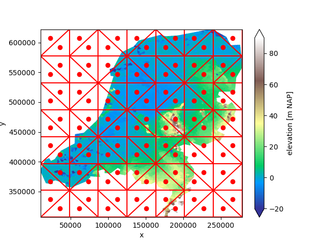
CentroidLocatorRegridder#
An easy way of regridding is by simply looking in which cell of the original the centroids of the new grid fall.
fig, ax = plt.subplots()
uda.ugrid.plot(vmin=-20, vmax=90, cmap="terrain", ax=ax)
grid.plot(ax=ax, color="red")
ax.scatter(*grid.centroids.T, color="red")
<matplotlib.collections.PathCollection object at 0x7fea65f6c320>
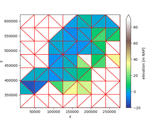
Xugrid provides the CentroidLocatorRegridder for this:
regridder = xu.CentroidLocatorRegridder(source=uda, target=grid)
result = regridder.regrid(uda)
result.ugrid.plot(vmin=-20, vmax=90, cmap="terrain", edgecolor="red")
<matplotlib.collections.PolyCollection object at 0x7feaafa61220>
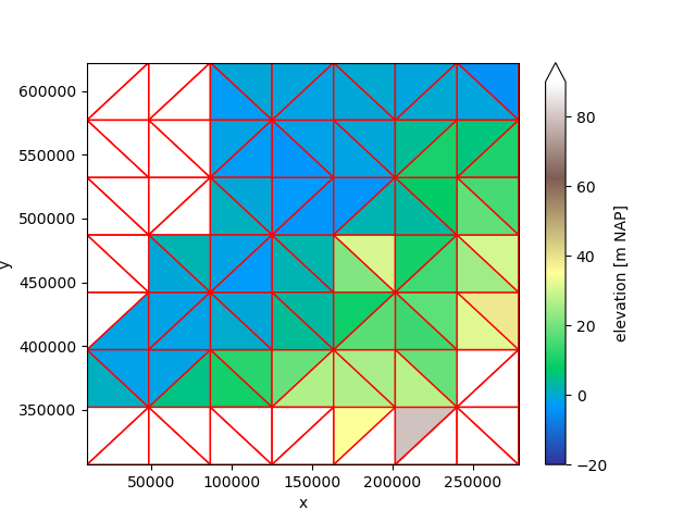
OverlapRegridder#
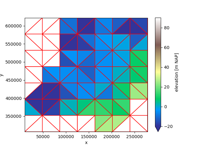
Such a regridding is not appropriate when the new grid cells are so large. Let’s try the OverlapOverregridder instead.
regridder = xu.OverlapRegridder(source=uda, target=grid)
mean = regridder.regrid(uda)
mean.ugrid.plot(vmin=-20, vmax=90, cmap="terrain", edgecolor="red")
<matplotlib.collections.PolyCollection object at 0x7fea64fc3410>
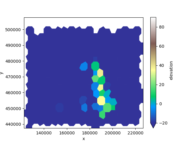
By default, the OverlapRegridder computes an area weighted mean. Let’s try again, now with the minimum:
regridder = xu.OverlapRegridder(source=uda, target=grid, method="minimum")
minimum = regridder.regrid(uda)
minimum.ugrid.plot(vmin=-20, vmax=90, cmap="terrain", edgecolor="red")
<matplotlib.collections.PolyCollection object at 0x7fea65bb9880>
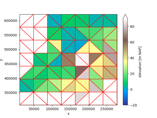
Or the maximum:
regridder = xu.OverlapRegridder(source=uda, target=grid, method="maximum")
maximum = regridder.regrid(uda)
maximum.ugrid.plot(vmin=-20, vmax=90, cmap="terrain", edgecolor="red")
<matplotlib.collections.PolyCollection object at 0x7fea65a77200>
All regridders also work for multi-dimensional data.
Let’s pretend our elevation dataset contains multiple layers, for example to denote multiple geological strata. We’ll generate five layers, each with a thickness of 10.0 meters.
thickness = xr.DataArray(
    data=[10.0, 10.0, 10.0, 10.0, 10.0],
    coords={"layer": [1, 2, 3, 4, 5]},
    dims=["layer"],
)
We need to make that the face dimension remains last, so we transpose the result.
bottom = (uda - thickness.cumsum("layer")).transpose()
bottom
We can feed the result to the regridder, which will automatically regrid over all additional dimensions.
mean_bottom = xu.OverlapRegridder(source=bottom, target=grid).regrid(bottom)
mean_bottom
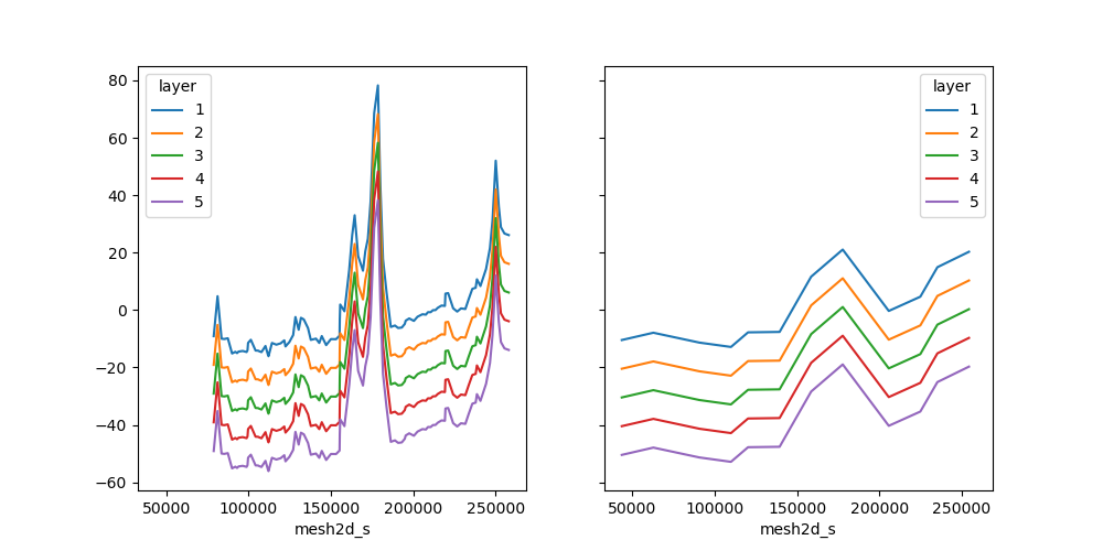
Let’s take a slice to briefly inspect our original layer bottom elevation, and the aggregated mean.
section_y = 475_000.0
section = bottom.ugrid.sel(y=section_y)
section_mean = mean_bottom.ugrid.sel(y=section_y)

fig, (ax0, ax1) = plt.subplots(ncols=2, figsize=(10, 5), sharex=True, sharey=True)
section.plot.line(x="mesh2d_s", hue="layer", ax=ax0)
section_mean.plot.line(x="mesh2d_s", hue="layer", ax=ax1)
[<matplotlib.lines.Line2D object at 0x7fea65a77890>, <matplotlib.lines.Line2D object at 0x7feaaf993a10>, <matplotlib.lines.Line2D object at 0x7feaaf992120>, <matplotlib.lines.Line2D object at 0x7feaaf9930e0>, <matplotlib.lines.Line2D object at 0x7feaaf993f20>]
BarycentricInterpolator#
All examples above show reductions: from a fine grid to a coarse grid. However, xugrid also provides interpolation to generate smooth fine representations of a coarse grid.
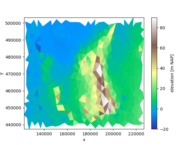
To illustrate, we will zoom in to a part of the Netherlands.
part = uda.ugrid.sel(x=slice(125_000, 225_000), y=slice(440_000, 500_000))
part.ugrid.plot(vmin=-20, vmax=90, cmap="terrain")
<matplotlib.collections.PolyCollection object at 0x7fea65b765d0>
We can clearly identify the individual triangles that form the grid. To get a smooth presentation, we can use the BarycentricInterpolator.
We will generate a fine grid.
grid = create_grid(part.ugrid.total_bounds, nx=100, ny=100)
We use the centroids of the fine grid to interpolate between the centroids of the triangles.
regridder = xu.BarycentricInterpolator(part, grid)
interpolated = regridder.regrid(part)
interpolated.ugrid.plot(vmin=-20, vmax=90, cmap="terrain")
<matplotlib.collections.PolyCollection object at 0x7fea65df7350>
Arbitrary grids#
The above examples all feature triangular source and target grids. However, the regridders work for any collection of (convex) faces.
grid = create_grid(part.ugrid.total_bounds, nx=20, ny=15)
voronoi_grid = grid.tesselate_centroidal_voronoi()

regridder = xu.CentroidLocatorRegridder(part, voronoi_grid)
result = regridder.regrid(part)

fig, ax = plt.subplots()
result.ugrid.plot(vmin=-20, vmax=90, cmap="terrain")
voronoi_grid.plot(ax=ax, color="red")
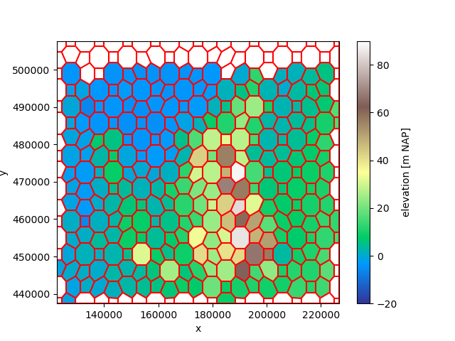
<matplotlib.collections.LineCollection object at 0x7fea65d09370>
Re-use#
The most expensive step of the regridding process is finding and computing overlaps. A regridder can be used repeatedly, provided the source topology is kept the same.
part_other = part - 50.0
result = regridder.regrid(part_other)
result.ugrid.plot(vmin=-20, vmax=90, cmap="terrain")
<matplotlib.collections.PolyCollection object at 0x7fea65c9b170>
Total running time of the script: (0 minutes 9.465 seconds)