Partitioning

Grid partitioning, or domain decomposition, is an important step in setting up parallellized simulations. Xugrid provides utilities for partitioning a grid and its associated data, and for merging partitions back into a single whole.

import matplotlib.pyplot as plt
import numpy as np

import xugrid as xu

Create partitions

Xugrid wraps the well known METIS library via the pymetis bindings. METIS is generally used to partition a grid in such a manner that communication between parallel processes is minimized.

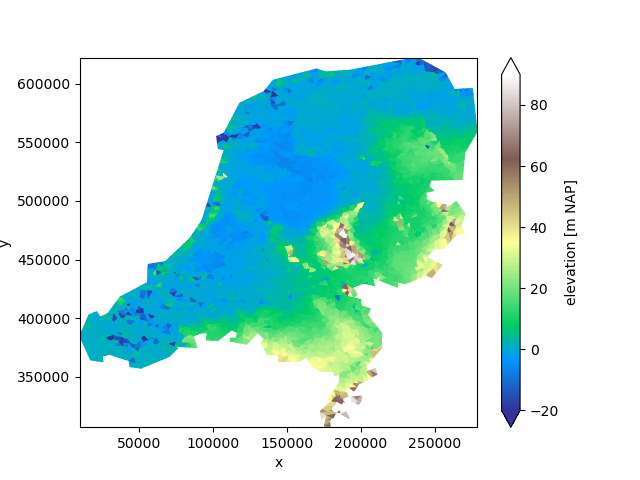
We’ll demonstrate the functionality by diving the elevation example into several parts.

uda = xu.data.elevation_nl()
uda.ugrid.plot(vmin=-20, vmax=90, cmap="terrain")

<matplotlib.collections.PolyCollection object at 0x7f604912d4f0>

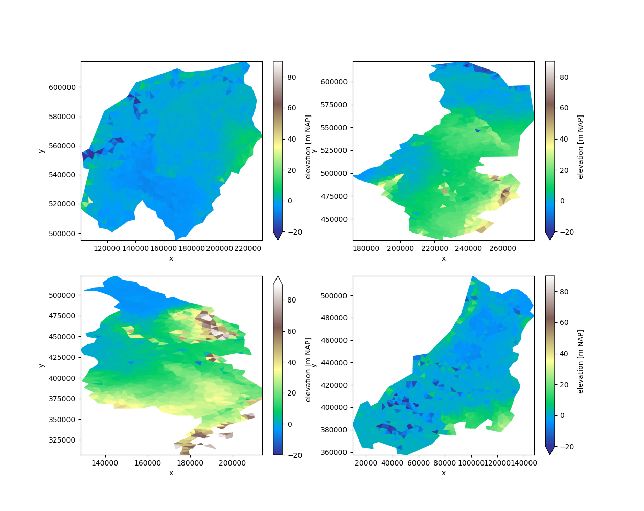
Let’s start by dividing the grid into four parts:

partitions = uda.ugrid.partition(n_part=4)

fig, axes = plt.subplots(2, 2, figsize=(12.6, 10))
for partition, ax in zip(partitions, axes.ravel()):
    partition.ugrid.plot(ax=ax, vmin=-20, vmax=90, cmap="terrain")

Partition the grid

Calling .partition on a UgridDataArray or UgridDataset will automatically partition the grid topology, select all associated data, and create a new UgridDataArray or UgridDataset for each partition.

However, in some case, we might prefer to pre-compute the labels, and then apply them multiple datasets. To do so, we compute the partition labels from the grid. label_partitions returns a UgridDataArray, with every cell given its partition label number.

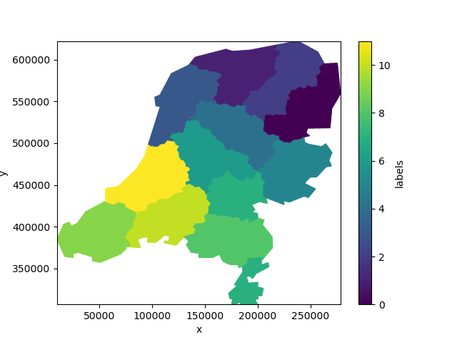
We can easily plot this data to visualize the partitions:

labels = uda.ugrid.grid.label_partitions(n_part=12)
labels.ugrid.plot()

<matplotlib.collections.PolyCollection object at 0x7f60513b8890>

Not quite the twelve provinces of the Netherlands!

However, we may use the labels to partition the data nonetheless:

partitions = uda.ugrid.partition_by_label(labels)

fig, axes = plt.subplots(4, 3, figsize=(15, 15))
for partition, ax in zip(partitions, axes.ravel()):
    partition.ugrid.plot(ax=ax, vmin=-20, vmax=90, cmap="terrain")

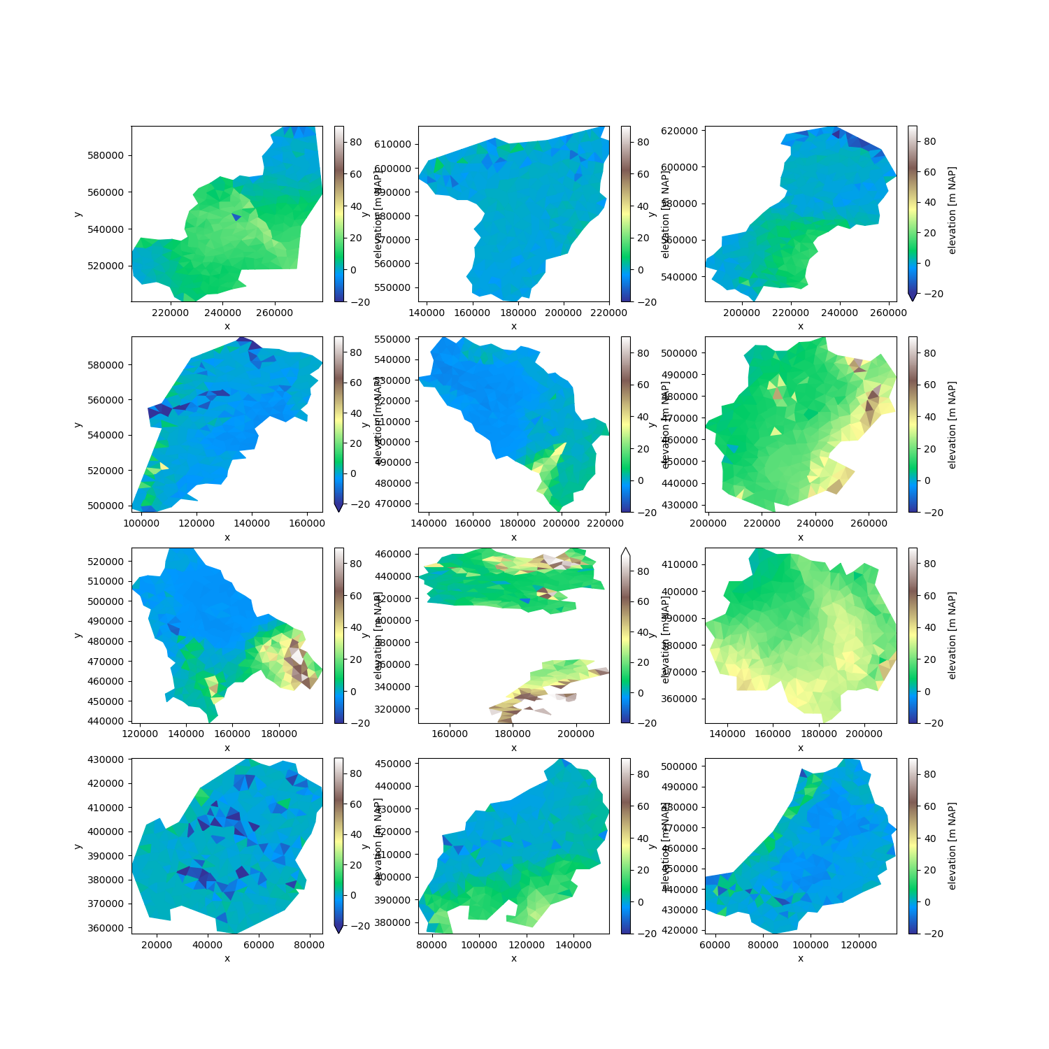
Since the labels are an ordinary UgridDataArray, we can easily store them in a netCDF file and re-use them in another part of a workflow.

Merging partitions

Generally, after partitioning the data we write it as model input and run a model in parallel. Many model codes produce output per process. Xugrid can merge these partitions back into one whole for post-processing:

merged = xu.merge_partitions(partitions)["elevation"]

merged.ugrid.plot(vmin=-20, vmax=90, cmap="terrain")

<matplotlib.collections.PolyCollection object at 0x7f60520d1010>

Partitioning grids without data

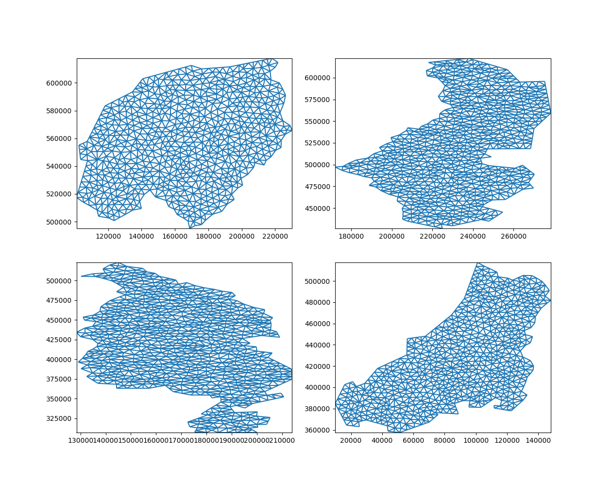
Of course, we can also partition the grid topology without any associated data:

grid = uda.ugrid.grid
grid_parts = grid.partition(n_part=4)

fig, axes = plt.subplots(2, 2, figsize=(12.6, 10))
for part, ax in zip(grid_parts, axes.ravel()):
    part.plot(ax=ax)

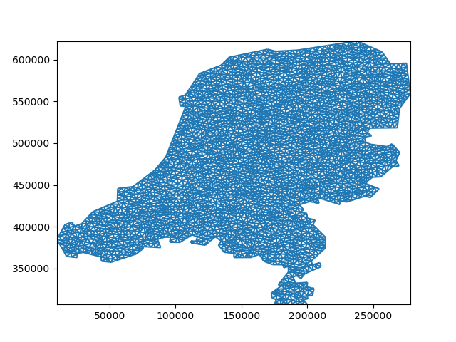
… and merge them back into one whole:

merged_grid, _ = xu.Ugrid2d.merge_partitions(grid_parts)
merged_grid.plot()

<matplotlib.collections.LineCollection object at 0x7f60479a6c60>

Preserving order

Note that partioning and merging does not preserve order!

uda == merged

<xarray.DataArray 'elevation' (mesh2d_nFaces: 5248)> Size: 5kB
array([False, False, False, ..., False, False, False])
Coordinates:
  * mesh2d_nFaces  (mesh2d_nFaces) int64 42kB 0 1 2 3 4 ... 5244 5245 5246 5247

xarray.DataArray

'elevation'

• mesh2d_nFaces: 5248

• False False False False False False ... False False False False False

  array([False, False, False, ..., False, False, False])

• Coordinates: (1)
  • mesh2d_nFaces
    (mesh2d_nFaces)
    int64
    0 1 2 3 4 ... 5244 5245 5246 5247

    array([   0,    1,    2, ..., 5245, 5246, 5247])

• Indexes: (1)
  • mesh2d_nFaces
    PandasIndex

    PandasIndex(RangeIndex(start=0, stop=5248, step=1, name='mesh2d_nFaces'))

• Attributes: (0)

The topology is equivalent, but the nodes, edges, and faces are in a different order. This is because merge_partitions simply concatenates the partitions.

The easiest way to restore the order is by providing an example of the original topology. reindex_like looks at the coordinates of both (equivalent!) grids and automatically determines how to reorder:

reordered = merged.ugrid.reindex_like(uda)
uda == reordered

<xarray.DataArray 'elevation' (mesh2d_nFaces: 5248)> Size: 5kB
array([ True,  True,  True, ...,  True,  True,  True])
Coordinates:
    mesh2d_face_x  (mesh2d_nFaces) float64 42kB 2.388e+04 1.86e+05 ... 3.03e+04
    mesh2d_face_y  (mesh2d_nFaces) float64 42kB 3.648e+05 ... 3.964e+05
  * mesh2d_nFaces  (mesh2d_nFaces) int64 42kB 0 1 2 3 4 ... 5244 5245 5246 5247

xarray.DataArray

'elevation'

• mesh2d_nFaces: 5248

• True True True True True True True ... True True True True True True

  array([ True,  True,  True, ...,  True,  True,  True])

• Coordinates: (3)
  • mesh2d_face_x
    (mesh2d_nFaces)
    float64
    2.388e+04 1.86e+05 ... 3.03e+04

    standard_name :

    projection_x_coordinate

    array([ 23882.79376058, 186048.98609163, 183280.61324667, ...,
            33842.56847139,  33139.63056206,  30303.5164253 ])

  • mesh2d_face_y
    (mesh2d_nFaces)
    float64
    3.648e+05 4.171e+05 ... 3.964e+05

    standard_name :

    projection_y_coordinate

    array([364821.96725663, 417102.96121876, 334623.01878379, ...,
           397494.51640391, 400187.85011645, 396399.29036318])

  • mesh2d_nFaces
    (mesh2d_nFaces)
    int64
    0 1 2 3 4 ... 5244 5245 5246 5247

    array([   0,    1,    2, ..., 5245, 5246, 5247])

• Indexes: (1)
  • mesh2d_nFaces
    PandasIndex

    PandasIndex(RangeIndex(start=0, stop=5248, step=1, name='mesh2d_nFaces'))

• Attributes: (0)

Alternatively, we can also assign IDs, carry these along, and use these to reorder the data after merging.

uds = xu.UgridDataset(grids=[uda.ugrid.grid])
uds["elevation"] = uda
uds["cell_id"] = ("mesh2d_nFaces", np.arange(len(uda)))

partitions = uds.ugrid.partition(n_part=4)
merged = xu.merge_partitions(partitions)
order = np.argsort(merged["cell_id"].values)
reordered = merged.isel(mesh2d_nFaces=order)

uds["elevation"] == reordered["elevation"]

<xarray.DataArray 'elevation' (mesh2d_nFaces: 5248)> Size: 5kB
array([ True,  True,  True, ...,  True,  True,  True])
Coordinates:
    mesh2d_face_x  (mesh2d_nFaces) float64 42kB 2.388e+04 1.86e+05 ... 3.03e+04
    mesh2d_face_y  (mesh2d_nFaces) float64 42kB 3.648e+05 ... 3.964e+05
  * mesh2d_nFaces  (mesh2d_nFaces) int64 42kB 0 1 2 3 4 ... 5244 5245 5246 5247

xarray.DataArray

'elevation'

• mesh2d_nFaces: 5248

• True True True True True True True ... True True True True True True

  array([ True,  True,  True, ...,  True,  True,  True])

• Coordinates: (3)
  • mesh2d_face_x
    (mesh2d_nFaces)
    float64
    2.388e+04 1.86e+05 ... 3.03e+04

    standard_name :

    projection_x_coordinate

    array([ 23882.79376058, 186048.98609163, 183280.61324667, ...,
            33842.56847139,  33139.63056206,  30303.5164253 ])

  • mesh2d_face_y
    (mesh2d_nFaces)
    float64
    3.648e+05 4.171e+05 ... 3.964e+05

    standard_name :

    projection_y_coordinate

    array([364821.96725663, 417102.96121876, 334623.01878379, ...,
           397494.51640391, 400187.85011645, 396399.29036318])

  • mesh2d_nFaces
    (mesh2d_nFaces)
    int64
    0 1 2 3 4 ... 5244 5245 5246 5247

    array([   0,    1,    2, ..., 5245, 5246, 5247])

• Indexes: (1)
  • mesh2d_nFaces
    PandasIndex

    PandasIndex(RangeIndex(start=0, stop=5248, step=1, name='mesh2d_nFaces'))

• Attributes: (0)

This is required if results are compared with the input, or with results stemming from another partitioning, e.g. one with a different number of partitions.