Vector geometry conversion

A great deal of geospatial data is available not in gridded form, but in vectorized form: as points, lines, and polygons. In the Python data ecosystem, these geometries and their associated data are generally represented by a geopandas GeoDataFrame.

Xugrid provides a number of utilities to use such data in combination with unstructured grids. These are demonstrated below.

import geopandas as gpd
import matplotlib.pyplot as plt
import pandas as pd

import xugrid as xu

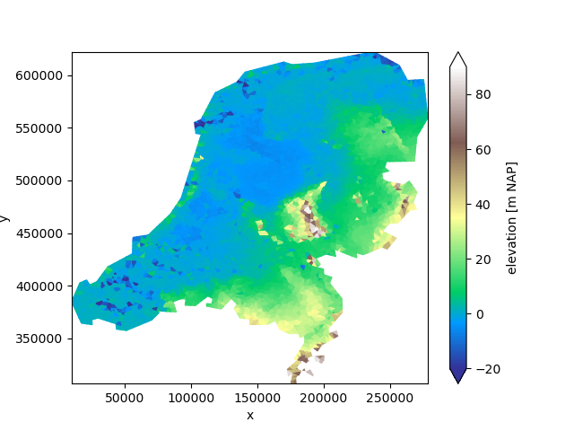
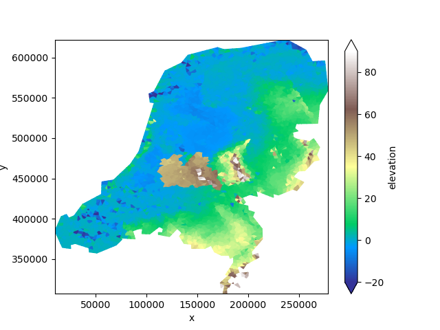
We’ll once again use the surface elevation data example.

uda = xu.data.elevation_nl()
uda.ugrid.plot(vmin=-20, vmax=90, cmap="terrain")

<matplotlib.collections.PolyCollection object at 0x7f98dfbb71a0>

Conversion to GeoDataFrame

A UgridDataArray or UgridDataset can be directly converted to a GeoDataFrame, provided it only contains a spatial dimension (and not a dimension such as time). When calling .to_geodataframe, a shapely Polygon is created for every face (cell).

gdf = uda.ugrid.to_geodataframe()
print(gdf)

               elevation  ...                                           geometry
mesh2d_nFaces             ...
0               1.170000  ...  POLYGON ((21303.903 363737.469, 25340.195 3630...
1               9.810000  ...  POLYGON ((185417.879 419222.681, 184927.836 41...
2              54.040001  ...  POLYGON ((181811.627 338063.592, 182510.446 33...
3               0.990000  ...  POLYGON ((20177.702 368500.703, 17210.674 3644...
4               2.600000  ...  POLYGON ((51139.349 357499.291, 48079.937 3617...
...                  ...  ...                                                ...
5243            0.930000  ...  POLYGON ((38115.173 400096.935, 34838.247 3952...
5244           36.189999  ...  POLYGON ((252916.585 467082.681, 255888.448 45...
5245            0.280000  ...  POLYGON ((34838.247 395258.331, 34522.298 3998...
5246          -15.830000  ...  POLYGON ((32729.434 403338.332, 32167.160 3973...
5247           -0.450000  ...  POLYGON ((29985.831 394355.220, 32167.160 3973...

[5248 rows x 4 columns]

We see that a GeoDataFrame with 5248 rows is created: one row for each face.

Conversion from GeoDataFrame

We can also make the opposite conversion: we can create a UgridDataSet from a GeoDataFrame.

back = xu.UgridDataset.from_geodataframe(gdf)
back

<xarray.Dataset> Size: 147kB
Dimensions:        (mesh2d_nFaces: 5248)
Coordinates:
  * mesh2d_nFaces  (mesh2d_nFaces) int64 42kB 0 1 2 3 4 ... 5244 5245 5246 5247
Data variables:
    elevation      (mesh2d_nFaces) float32 21kB 1.17 9.81 54.04 ... -15.83 -0.45
    mesh2d_face_x  (mesh2d_nFaces) float64 42kB 2.388e+04 1.86e+05 ... 3.03e+04
    mesh2d_face_y  (mesh2d_nFaces) float64 42kB 3.648e+05 ... 3.964e+05

xarray.Dataset

• Dimensions:
  • mesh2d_nFaces: 5248
• Coordinates: (1)
  • mesh2d_nFaces
    (mesh2d_nFaces)
    int64
    0 1 2 3 4 ... 5244 5245 5246 5247

    array([   0,    1,    2, ..., 5245, 5246, 5247])

• Data variables: (3)
  • elevation
    (mesh2d_nFaces)
    float32
    1.17 9.81 54.04 ... -15.83 -0.45

    array([  1.17,   9.81,  54.04, ...,   0.28, -15.83,  -0.45], dtype=float32)

  • mesh2d_face_x
    (mesh2d_nFaces)
    float64
    2.388e+04 1.86e+05 ... 3.03e+04

    array([ 23882.79376058, 186048.98609163, 183280.61324667, ...,
            33842.56847139,  33139.63056206,  30303.5164253 ])

  • mesh2d_face_y
    (mesh2d_nFaces)
    float64
    3.648e+05 4.171e+05 ... 3.964e+05

    array([364821.96725663, 417102.96121876, 334623.01878379, ...,
           397494.51640391, 400187.85011645, 396399.29036318])

• Indexes: (1)
  • mesh2d_nFaces
    PandasIndex

    PandasIndex(RangeIndex(start=0, stop=5248, step=1, name='mesh2d_nFaces'))

• Attributes: (0)

Note

Not every GeoDataFrame can be converted to a xugrid representation! While an unstructured grid topology is generally always a valid collection of polygon geometries, not every collection of polygon geometries is a valid grid: polygons should be convex and non-overlapping to create a valid unstructured grid.

Secondly, each polygon fully owns its vertices (nodes), while the face of a UGRID topology shares its nodes with its neighbors. All the vertices of the polygons must therefore be exactly snapped together to form a connected mesh.

Hence, the .from_geodataframe() is primarily meant to create xugrid objects from data that were originally created as triangulation or unstructured grid, but that were converted to vector geometry form.

“Rasterizing”, or “burning” vector geometries

Rasterizing is a common operation when working with raster and vector data. While we cannot name the operation “rasterizing” when we’re dealing with unstructured grids, there is a clearly equivalent operation where we mark cells that are covered or touched by a polygon.

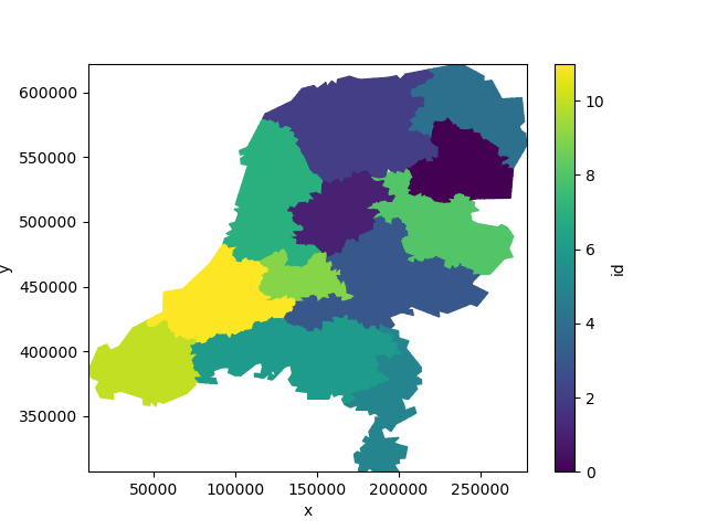
In this example, we mark the faces that are covered by a certain province.

We start by re-projecting the provinces dataset to the coordinate reference system (CRS), from WGS84 (EPSG:4326) to the Dutch National coordinate system (RD New, EPSG: 28992). Then, we give each province a unique id, which we burn into the grid.

provinces = xu.data.provinces_nl().to_crs(28992)
provinces["id"] = range(len(provinces))
burned = xu.burn_vector_geometry(provinces, uda, column="id")
burned.ugrid.plot()

<matplotlib.collections.PolyCollection object at 0x7f98e0033b00>

This makes it very easy to classify and group data. Let’s say we want to compute the average surface elevation per province:

burned = xu.burn_vector_geometry(provinces, uda, column="id")
uda.groupby(burned).mean()

<xarray.DataArray 'elevation' (id: 12)> Size: 48B
array([10.725979  , -3.806918  , -0.46903867, 17.090816  ,  0.3133026 ,
       52.252567  , 12.194658  , -1.7175047 , 11.021334  ,  3.0442472 ,
       -1.4584134 , -0.9470762 ], dtype=float32)
Coordinates:
  * id       (id) float64 96B 0.0 1.0 2.0 3.0 4.0 5.0 6.0 7.0 8.0 9.0 10.0 11.0
Attributes:
    unit:     m NAP

xarray.DataArray

'elevation'

• id: 12

• 10.73 -3.807 -0.469 17.09 0.3133 ... -1.718 11.02 3.044 -1.458 -0.9471

  array([10.725979  , -3.806918  , -0.46903867, 17.090816  ,  0.3133026 ,
         52.252567  , 12.194658  , -1.7175047 , 11.021334  ,  3.0442472 ,
         -1.4584134 , -0.9470762 ], dtype=float32)

• Coordinates: (1)
  • id
    (id)
    float64
    0.0 1.0 2.0 3.0 ... 9.0 10.0 11.0

    array([ 0.,  1.,  2.,  3.,  4.,  5.,  6.,  7.,  8.,  9., 10., 11.])

• Indexes: (1)
  • id
    PandasIndex

    PandasIndex(Index([0.0, 1.0, 2.0, 3.0, 4.0, 5.0, 6.0, 7.0, 8.0, 9.0, 10.0, 11.0], dtype='float64', name='id'))

• Attributes: (1)

  unit :

  m NAP

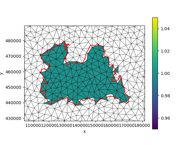
This is a convenient way to create masks for specific regions:

utrecht = provinces[provinces["name"] == "Utrecht"]
burned = xu.burn_vector_geometry(utrecht, uda)
xmin, ymin, xmax, ymax = utrecht.buffer(10_000).total_bounds

fig, ax = plt.subplots()
burned.ugrid.plot(ax=ax)
burned.ugrid.plot.line(ax=ax, edgecolor="black", linewidth=0.5)
utrecht.plot(ax=ax, edgecolor="red", facecolor="none", linewidth=1.5)
ax.set_xlim(xmin, xmax)
ax.set_ylim(ymin, ymax)

(428343.70545104187, 489587.5779869387)

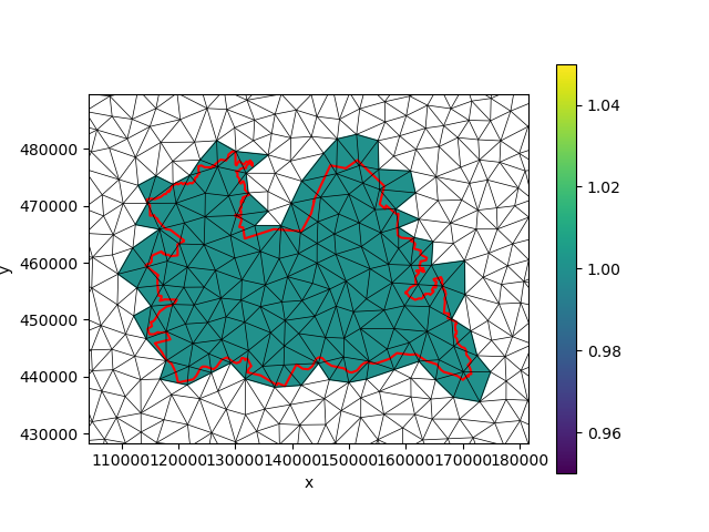
By default, burn_vector_geometry will only include grid faces whose centroid are located in a polygon. We can also mark all intersected faces by setting all_touched=True:

burned = xu.burn_vector_geometry(utrecht, uda, all_touched=True)

fig, ax = plt.subplots()
burned.ugrid.plot(ax=ax)
burned.ugrid.plot.line(ax=ax, edgecolor="black", linewidth=0.5)
utrecht.plot(ax=ax, edgecolor="red", facecolor="none", linewidth=1.5)
ax.set_xlim(xmin, xmax)
ax.set_ylim(ymin, ymax)

(428343.70545104187, 489587.5779869387)

We can also use such “masks” to e.g. modify specific parts of the grid data:

modified = (uda + 50.0).where(burned == 1, other=uda)
modified.ugrid.plot(vmin=-20, vmax=90, cmap="terrain")

<matplotlib.collections.PolyCollection object at 0x7f98ea9d9070>

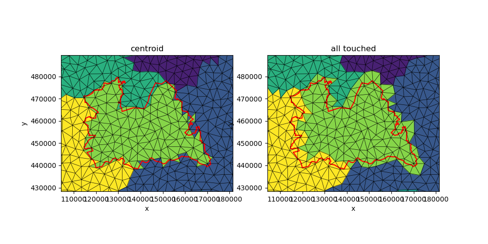
Note that all_touched=True is less suitable when differently valued polygons are present that share borders. While the centroid of a face is contained by only a single polygon, the area of the polygon may be located in more than one polygon. In this case, the results of each polygon will overwrite each other.

by_centroid = xu.burn_vector_geometry(provinces, uda, column="id")
by_touch = xu.burn_vector_geometry(provinces, uda, column="id", all_touched=True)

fig, axes = plt.subplots(ncols=2, figsize=(10, 5))
by_centroid.ugrid.plot(ax=axes[0], add_colorbar=False)
by_touch.ugrid.plot(ax=axes[1], add_colorbar=False)

for ax, title in zip(axes, ("centroid", "all touched")):
    burned.ugrid.plot.line(ax=ax, edgecolor="black", linewidth=0.5)
    utrecht.plot(ax=ax, edgecolor="red", facecolor="none", linewidth=1.5)
    ax.set_xlim(xmin, xmax)
    ax.set_ylim(ymin, ymax)
    ax.set_title(title)

This function can also be used to burn points or lines into the faces of an unstructured grid.

The exterior boundaries of the province polygons will provide a collection of linestrings that we can burn into the grid:

lines = gpd.GeoDataFrame(geometry=provinces.exterior)
burned = xu.burn_vector_geometry(lines, uda)

fig, ax = plt.subplots()
burned.ugrid.plot(ax=ax)
burned.ugrid.plot.line(ax=ax, edgecolor="black", linewidth=0.5)
provinces.plot(ax=ax, edgecolor="red", facecolor="none", linewidth=1.5)
ax.set_xlim(xmin, xmax)
ax.set_ylim(ymin, ymax)

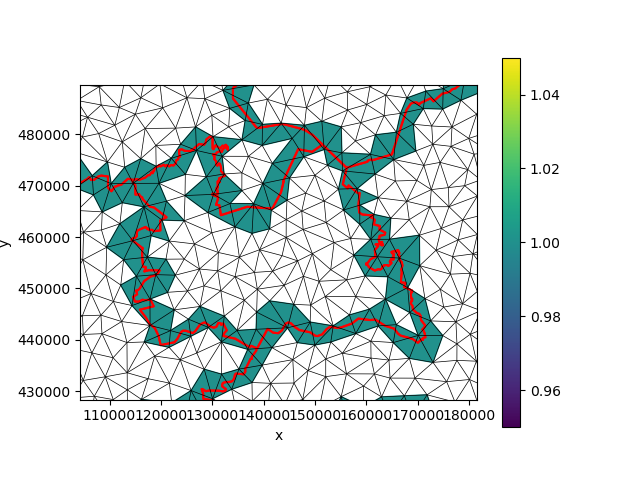
(428343.70545104187, 489587.5779869387)

We can also burn points.

province_centroids = gpd.GeoDataFrame(geometry=provinces.centroid)
burned = xu.burn_vector_geometry(province_centroids, uda)

fig, ax = plt.subplots()
burned.ugrid.plot(ax=ax)
provinces.plot(ax=ax, edgecolor="red", facecolor="none")

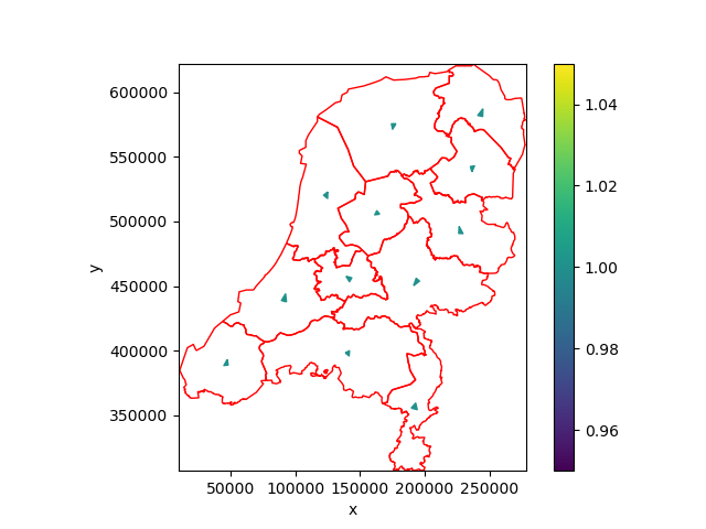
<Axes: xlabel='x', ylabel='y'>

Finally, it’s also possible to combine multiple geometry types in a single burn operation.

combined = pd.concat([lines, province_centroids])
burned = xu.burn_vector_geometry(combined, uda)
burned.ugrid.plot()

<matplotlib.collections.PolyCollection object at 0x7f98da7ba6f0>

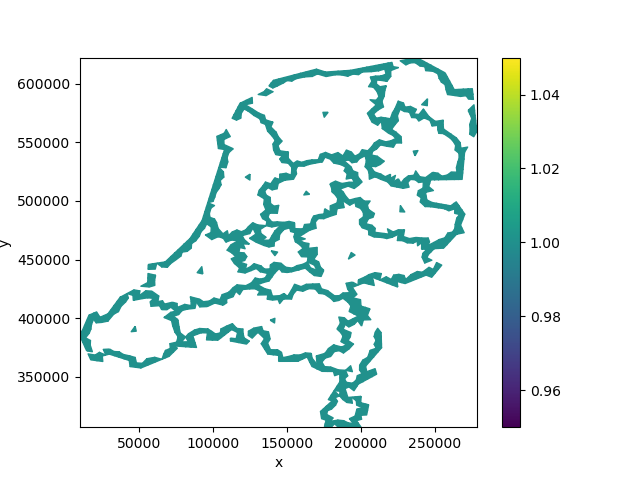
Polygonizing

We can also do the opposite operation: turn collections of same-valued grid faces into vector polygons. Let’s classify the elevation data into below and above the boundary of 5 m above mean sea level:

classified = uda > 5
polygonized = xu.polygonize(classified)
polygonized.plot(facecolor="none")

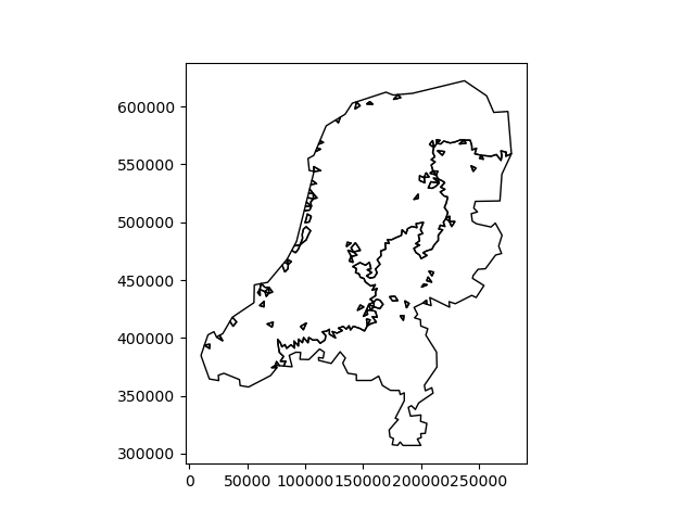
<Axes: >

We see that the results consists of two large polygons, in which the triangles of the triangular grid have been merged to form a single polygon, and many smaller polygons, some of which correspond one to one to the triangles of the grid.

Note

The produced polygon edges will follow exactly the face boundaries. When the data consists of many unique values (e.g. unbinned elevation data), the result will essentially be one polygon per face. In such cases, it is more efficient to use xugrid.UgridDataArray.to_geodataframe, which directly converts every face to a polygon.

Snap to grid

The examples above deal with data on the faces of the grid. However, data can also be associated with the nodes or edges of the grid. For example, we can snap line data to exactly follow the edges (the face boundaries):

linestrings = gpd.GeoDataFrame(geometry=utrecht.exterior)
snapped_uds, snapped_gdf = xu.snap_to_grid(linestrings, uda, max_snap_distance=1.0)

fig, ax = plt.subplots()
snapped_gdf.plot(ax=ax)
snapped_uds.ugrid.grid.plot(ax=ax, edgecolor="gray", linewidth=0.5)
utrecht.plot(ax=ax, edgecolor="red", facecolor="none", linewidth=0.75)
ax.set_xlim(xmin, xmax)
ax.set_ylim(ymin, ymax)

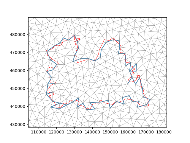
(428343.70545104187, 489587.5779869387)

There are (arguably) many ways in which a linestring could be snapped to edges. The function above uses the criterion the following criterion: if a part of the linestring is located between the centroid of a face and the centroid of an edge, it is snapped to that edge.

This sometimes result in less (visually) pleasing results, such as the two triangles in the lower left corner which are surrounded by the snapped edges. In general, results are best when the line segments are relatively large compare to the grid faces.