Note
Go to the end to download the full example code.
Plot unstructured mesh data#
The labels that are present in xarray’s data structures allow for easy creation of informative plots: think of dates on the x-axis, or geospatial coordinates. Xarray provides a convenient way of plotting your data provided it is structured. Xugrid extends these plotting methods to easily make spatial (x-y) plots of unstructured grids.
Like Xarray’s focus for plotting is the DataArray, Xugrid’s focus is the UgridDataArray; like Xarray, if your (extracted) data fits into a pandas DataFrame, you’re better of using pandas tools instead.
As every other method in Xugrid, any logic involving the unstructured topology
is accessed via the .ugrid accessor on the DataArrays and Datasets;
UgridDatasets and UgridDataArrays behave the same as ordinary Xarray DataArrays
and Datasets otherwise.
Imports#
The following imports suffice for the examples.
import matplotlib.pyplot as plt

import xugrid
We’ll use a simple synthetic example. This dataset contains data for all topological attributes of a two dimensional mesh:
Nodes: the coordinate pair (x, y) forming a point.
Edges: a line or curve bounded by two nodes.
Faces: the polygon enclosed by a set of edges.
In this disk example, very similar has been placed on the nodes, edges, and faces.
ds = xugrid.data.disk()
ds
UgridDataArray#
Just like Xarray, we can create a plot by selecting a DataArray from the
Dataset and calling the UgridDataArray.ugrid.plot() method.
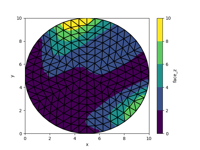
uda = ds["face_z"]
uda.ugrid.plot()
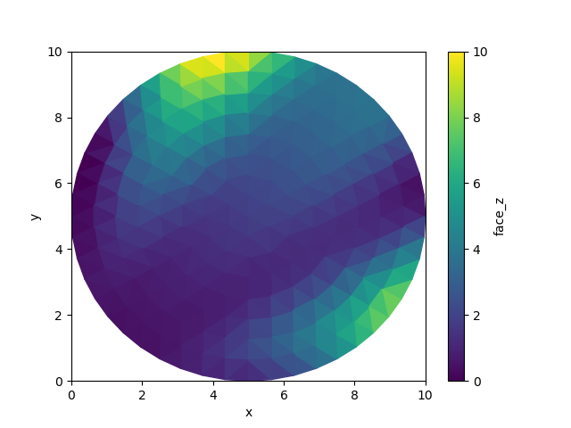
<matplotlib.collections.PolyCollection object at 0x7fea65b3a810>
Like Xarray, the axes and the colorbar are labeled automatically using the available information.
The convenience function xugrid.UgridDataArray.ugrid.plot()
dispatches on the topological dimension of the variable. In this case, the
data is associated with the face dimension of the topology. Data located on
the edges results in a different kind of plot:
ds["edge_z"].ugrid.plot()
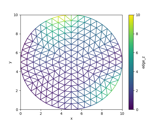
<matplotlib.collections.LineCollection object at 0x7feaaed365d0>
The method called by default depends on the type of the data:
Dimension |
Plotting function |
|---|---|
Face |
|
Edge |
|
Node |
We can put them side by side to illustrate the differences:
fig, (ax0, ax1, ax2) = plt.subplots(ncols=3, figsize=(11, 3), sharex=True, sharey=True)
ds["face_z"].ugrid.plot(ax=ax0)
ds["edge_z"].ugrid.plot(ax=ax1)
ds["node_z"].ugrid.plot(ax=ax2)
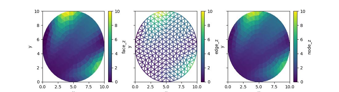
<matplotlib.collections.PolyCollection object at 0x7feaaed35430>
We can also exactly control the type of plot we want. For example, to plot filled contours for data associated with the face dimension:
ds["face_z"].ugrid.plot.contourf()
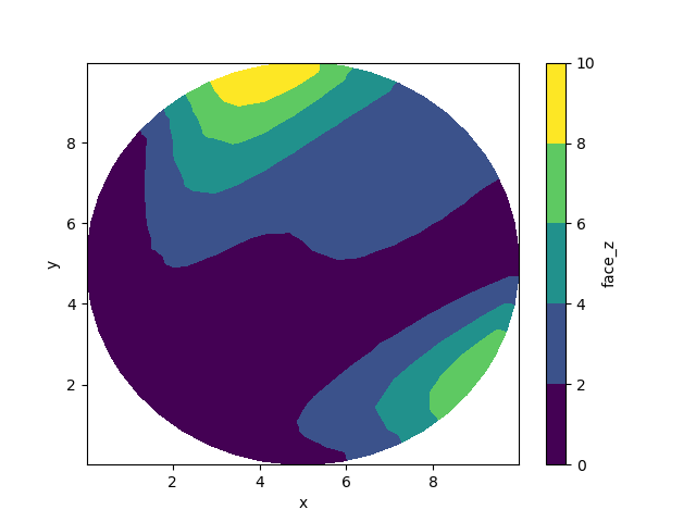
<matplotlib.tri._tricontour.TriContourSet object at 0x7fea65e69d00>
We can also overlay this data with the edges:
fig, ax = plt.subplots()
ds["face_z"].ugrid.plot.contourf()
ds["face_z"].ugrid.plot.line(color="black")
<matplotlib.collections.LineCollection object at 0x7feaafc48440>
In general, there has to be data associated with the mesh topology before a
plot can be made. plot.line() forms an exception to this rule, as the
location of the edges is meaningful on its own: for this reason
plot.line() does not error in the example above.
Other types of plot#
The available plotting methods per topology dimension are listed here.
For the face dimension:
For the edge dimension:
For the node dimension:
All these (2D) plots are illustrated here for completeness’ sake:
fig, axes = plt.subplots(nrows=5, ncols=3, figsize=(10, 15))

ds["face_z"].ugrid.plot.pcolormesh(ax=axes[0, 0])
ds["face_z"].ugrid.plot.contour(ax=axes[1, 0])
ds["face_z"].ugrid.plot.contourf(ax=axes[2, 0])
ds["face_z"].ugrid.plot.imshow(ax=axes[3, 0])
ds["face_z"].ugrid.plot.scatter(ax=axes[4, 0])

ds["edge_z"].ugrid.plot.line(ax=axes[0, 1])
ds["edge_z"].ugrid.plot.scatter(ax=axes[4, 1])

ds["node_z"].ugrid.plot.tripcolor(ax=axes[0, 2])
ds["node_z"].ugrid.plot.contour(ax=axes[1, 2])
ds["node_z"].ugrid.plot.contourf(ax=axes[2, 2])
ds["node_z"].ugrid.plot.scatter(ax=axes[4, 2])
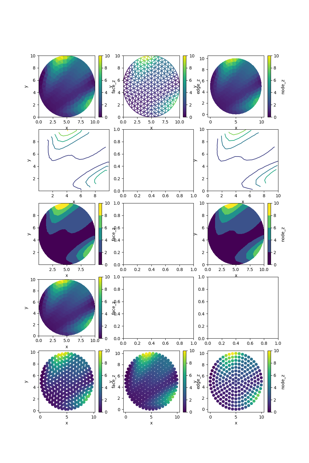
<matplotlib.collections.PathCollection object at 0x7fea64a879b0>
The surface methods generate 3D surface plots:
fig = plt.figure(figsize=plt.figaspect(0.5))
ax0 = fig.add_subplot(1, 2, 1, projection="3d")
ax1 = fig.add_subplot(1, 2, 2, projection="3d")
ds["face_z"].ugrid.plot.surface(ax=ax0)
ds["node_z"].ugrid.plot.surface(ax=ax1)
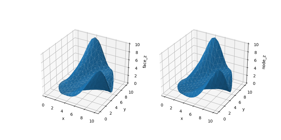
<mpl_toolkits.mplot3d.art3d.Poly3DCollection object at 0x7fea65b39340>
Additional Arguments#
Once again like in Xarray, additional arguments are passed to the underlying matplotlib function and the additional arguments supported by Xarray can be used:
ds["face_z"].ugrid.plot(cmap="RdBu", levels=8, yincrease=False)
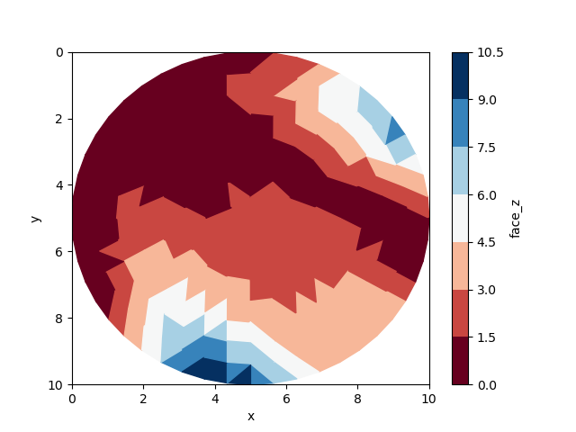
<matplotlib.collections.PolyCollection object at 0x7feaaec73170>
As a function#
The plotting methods can also be called as a function, in which case they take an xarray DataArray and a xugrid grid as arguments.
grid = ds.ugrid.grids[0]
da = ds.obj["face_z"]

xugrid.plot.pcolormesh(grid, da)

<matplotlib.collections.PolyCollection object at 0x7fea65b39ee0>
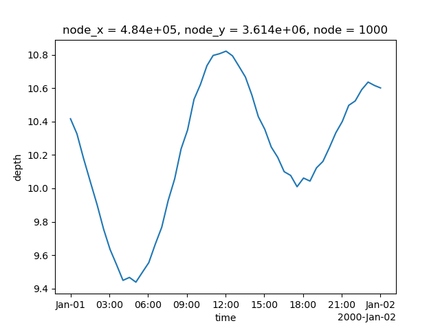
Xarray DataArray plots#
As mentioned, apart from the .ugrid accessor, a UgridDataArray behaves the
same as an Xarray DataArray. To illustrate, we can select a location
somewhere in the unstructured topology, and plot the resulting timeseries:
ds = xugrid.data.adh_san_diego()
depth = ds["depth"]
depth.isel(node=1000).plot()
[<matplotlib.lines.Line2D object at 0x7fea65c35c40>]
Total running time of the script: (0 minutes 15.183 seconds)