Connectivity

A fundamental difference between structured and unstructured grids lies in the connectivity. This is true for cell to cell connectivity, but also for vertex (node) connectivity (which set of vertices make up an individual cell). In structured grids, connectivity is implicit and can be directly derived from row and column numbers; unstructured grids require explicit connectivity lists.

Xugrid provides a number of methods to derive and extract different kinds of connectivities, as well as a number of operations which require connectivity information. These methods and their interrelations are briefly introduced here.

For 2D meshes, the fundamental topological information consists of:

• A list of nodes (vertices): (x, y) coordinate pairs forming points.

• A list of faces (polygons): for every face, a list of index values indicating which vertices form its exterior.

Imports

The following imports suffice for the examples.

import matplotlib.pyplot as plt
import numpy as np
import xarray as xr

import xugrid

Connectivity arrays

From the fundamental face node connectivity, all other connectivities can be derived. These are accessible via the grid attribute of a XugridDataArray or XugridDataset. The are the available (derived) connectivity arrays are listed below. Depending on the (ir)regularity of the connectivity, the arrays are returned as either (dense) numpy arrays of integers, or as scipy.sparse.csr_matrix.

• face_node_connectivity: dense (n_face, n_max_nodes_per_face)

• edge_node_connectivity: dense (n_edge, 2)

• edge_face_connectivity: dense (n_edge, 2)

• face_face_connectivity: sparse

• face_edge_connectivity: sparse

• node_edge_connectivity: sparse

• node_face_connectivity: sparse

Some connectivity arrays are returned in dense form, some in sparse. The node_edge_connectivity is the inverse of the edge_node_connectivity. While the edge node connectivity array is very regular – every edge is associated with just two nodes, the node edge connectivity is irregular: a node may be associated with just one edge or many and this requires many fill values in dense form.

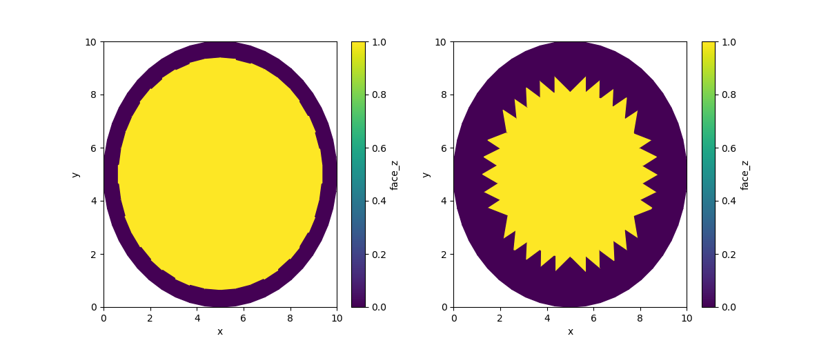
Binary erosion and dilation

Binary erosion and dilation are useful operations to e.g. locate boundary cells, or to “shrink” some collection of cells. In this example, we start with a grid in which all cells are given a value of True (equal to 1).

By default, the border value for binary erosion is set to False (equal to 0). This means the erosion erodes inwards from the boundaries.

ds = xugrid.data.disk()
uda = xugrid.UgridDataArray(
    xr.full_like(ds.obj["face_z"], True, dtype=bool),
    ds.grids[0],
)
iter2 = uda.ugrid.binary_erosion(iterations=2)
iter5 = uda.ugrid.binary_erosion(iterations=5)

fig, (ax0, ax1) = plt.subplots(ncols=2, figsize=(12, 5))
iter2.ugrid.plot(ax=ax0)
iter5.ugrid.plot(ax=ax1)

<matplotlib.collections.PolyCollection object at 0x7f98def00200>

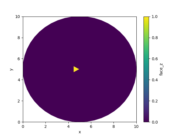
By default, the border value for binary dilation is also set to False. This means boundary does not dilate inwards by default. We’ll start by setting a single value in the center of the grid to True.

uda = xugrid.UgridDataArray(
    xr.full_like(ds["face_z"].ugrid.obj, False, dtype=bool),
    ds.grids[0],
)
uda[0] = True
uda.ugrid.plot()

<matplotlib.collections.PolyCollection object at 0x7f98dfe3ecc0>

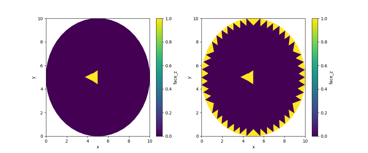
Now let’s run two dilations: one with the default border, and one with the alternative border value:

iter1 = uda.ugrid.binary_dilation(iterations=1)
iter1_boundary = uda.ugrid.binary_dilation(iterations=1, border_value=True)

fig, (ax0, ax1) = plt.subplots(ncols=2, figsize=(12, 5))
iter1.ugrid.plot(ax=ax0)
iter1_boundary.ugrid.plot(ax=ax1)

<matplotlib.collections.PolyCollection object at 0x7f98dfa09be0>

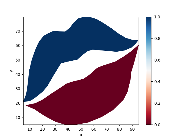
Connected Components

Xugrid also wraps scipy.sparse.csgraph.connected_components() to analyse connected parts of the mesh.

grid = xugrid.data.xoxo()
uda = xugrid.UgridDataArray(
    xr.DataArray(np.ones(grid.node_face_connectivity.shape[0]), dims=["face"]), grid
)
labeled = uda.ugrid.connected_components()
labeled.ugrid.plot(cmap="RdBu")

<matplotlib.collections.PolyCollection object at 0x7f98dfb86cc0>

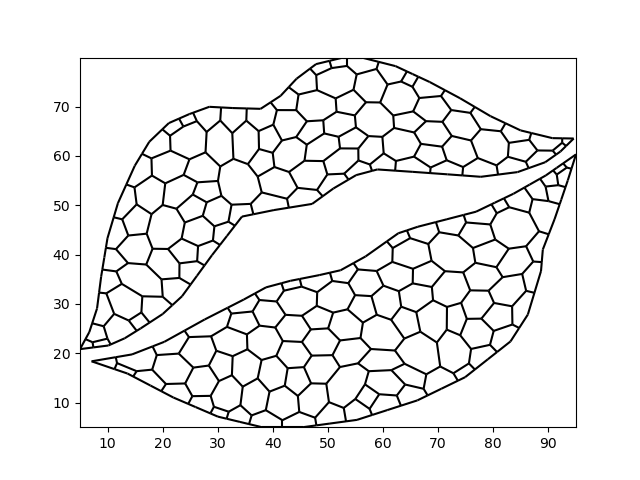
Centroidal Voronoi Tesselation

We can also use connectivity information to derive a centroidal Voronoi Tesselation.

voronoi_grid = grid.tesselate_centroidal_voronoi()
xugrid.plot.line(voronoi_grid, color="black")

<matplotlib.collections.LineCollection object at 0x7f98e0077170>

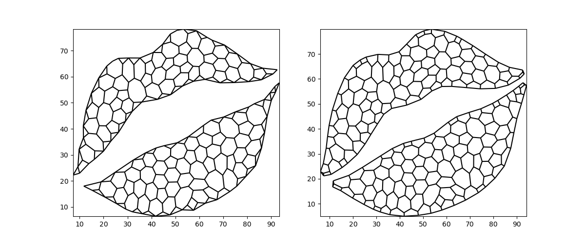
There are two alternative flavors to consider. We can fully ignore the exterior and consider only the (interior) centroids. Alternatively, we can include intersections of the voronoi edges with the mesh exterior, but ignore the original nodes.

Both methods have the benefit of guaranteeing convex Voronoi polygons as their output – provided the input mesh is convex as well! However, neither preserves the exterior exactly: the resulting mesh has smaller bounds than the original.

centroid_only = grid.tesselate_centroidal_voronoi(add_exterior=False)
convex_exterior = grid.tesselate_centroidal_voronoi(
    add_exterior=True, add_vertices=False
)

fig, (ax0, ax1) = plt.subplots(ncols=2, figsize=(12, 5))
xugrid.plot.line(centroid_only, ax=ax0, color="black")
xugrid.plot.line(convex_exterior, ax=ax1, color="black")

<matplotlib.collections.LineCollection object at 0x7f98dfbf39e0>

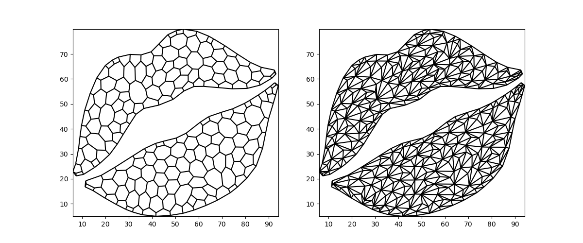
Triangulation

Triangulation is a commonly required operation: every polygon can be split into triangles and triangles are the simplest geometric primitive. This makes them very attractive for e.g. visualization.

We can break down one of the Voronoi tesselations from above into triangles:

triangulation = convex_exterior.triangulate()
fig, (ax0, ax1) = plt.subplots(ncols=2, figsize=(12, 5))
xugrid.plot.line(convex_exterior, ax=ax0, color="black")
xugrid.plot.line(triangulation, ax=ax1, color="black")

<matplotlib.collections.LineCollection object at 0x7f98df852d50>

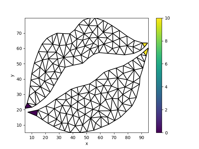
Laplace interpolation

Laplace interpolation is a simple but powerful method to fill holes in a grid. Laplace’s equation describes potential flow, such as e.g. steady-state heat conduction or steady-state groundwater flow. In this method, we solve Laplace’s equation for the nodata gaps, with data values functioning as fixed potential boundary conditions.

Let’s setup a mesh with data exclusively on the left- and rightmost faces of the upper and lower parts:

grid = xugrid.data.xoxo()

da = xr.DataArray(
    np.full(283, np.nan),
    dims=[grid.face_dimension],
)
da.data[2] = 0.0
da.data[12] = 0.0
da.data[77] = 10.0
da.data[132] = 10.0

uda = xugrid.UgridDataArray(da, grid)

fig, ax = plt.subplots()
uda.ugrid.plot(ax=ax)
uda.ugrid.plot.line(ax=ax, color="black")

<matplotlib.collections.LineCollection object at 0x7f98df944920>

We can now use Laplace interpolation to fill the gaps in the grid.

filled = uda.ugrid.laplace_interpolate()
filled.ugrid.plot(cmap="gist_rainbow", vmin=2.5, vmax=7.5)

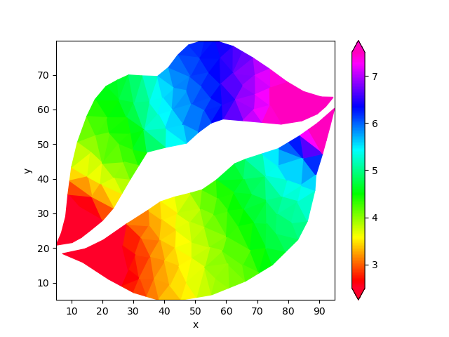
<matplotlib.collections.PolyCollection object at 0x7f98dfed2060>

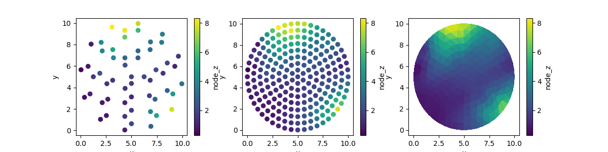
Laplace interpolation can also be used on the nodes of a grid. We start by removing 75% of the data. Then we fill it up again using interpolation.

disk_nodes = xugrid.data.disk()["node_z"]
disk_emptied = disk_nodes.where(disk_nodes["mesh2d_nNodes"] % 4 == 0)
disk_filled = disk_emptied.ugrid.laplace_interpolate(direct_solve=True)

fig, (ax0, ax1, ax2) = plt.subplots(ncols=3, figsize=(12, 3))
disk_emptied.ugrid.plot.scatter(ax=ax0)
disk_filled.ugrid.plot.scatter(ax=ax1)
disk_filled.ugrid.plot(ax=ax2)

<matplotlib.collections.PolyCollection object at 0x7f98dfefdf40>

Reverse-Cuthill McKee

For numerical solutions, low “bandwidth” is desirable as this increases performance due to more efficient memory access. Xugrid wraps scipy.sparse.csgraph.reverse_cuthill_mckee() to reorder grids for bandwith reduction.

To illustrate, let’s take a look at the connectivity matrix of the Xoxo grid.

grid = xugrid.data.xoxo()
connectivity = grid.face_face_connectivity.toarray() != 0

fig, ax = plt.subplots(figsize=(8, 8))
ax.imshow(connectivity, cmap="Greys")

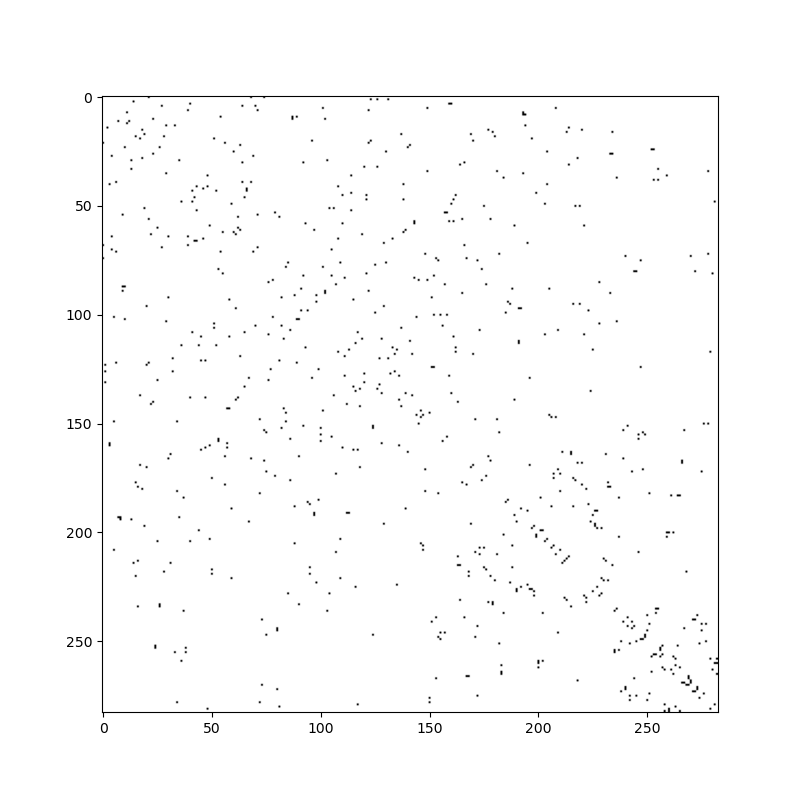
<matplotlib.image.AxesImage object at 0x7f98dfeaade0>

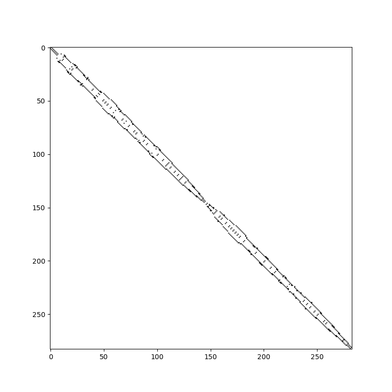
The bandwidth of this matrix is poor. Connections are all over the place: low numbered cells are connected to high numbered cells (and vice versa). The bandwidth of the reordered grid is much smaller and has much better data locality:

renumbered_grid, _ = grid.reverse_cuthill_mckee()
connectivity = renumbered_grid.face_face_connectivity.toarray() != 0

fig, ax = plt.subplots(figsize=(8, 8))
ax.imshow(connectivity, cmap="Greys")

<matplotlib.image.AxesImage object at 0x7f98dfec32f0>