Operations on distribution functions

In this example, we demonstrate various operations on distribution functions using the probabilistic library.

Define a stochastic variable

First, we import the necessary classes:

from probabilistic_library import DistributionType, Stochast, StandardNormal

Next, we create a random variable using the Stochast class:

stochast = Stochast()

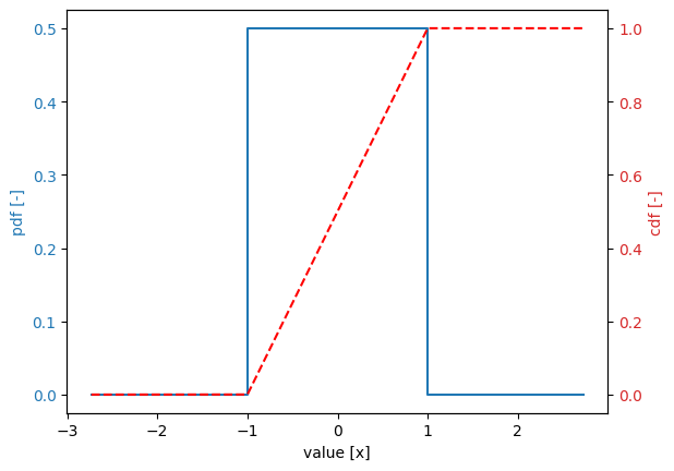
Let’s consider a random variable, which is uniformly distributed over the interval \([-1, 1]\). This is defined as follows:

stochast.distribution = DistributionType.uniform
stochast.minimum = -1
stochast.maximum = 1

stochast.plot()

The properties of this distribution are the minimum and maximum values, but also the derived properties as mean, deviation and coefficient of variation (variation):

stochast.print()

Variable:
  distribution = uniform
Definition:
  minimum = -1.0
  maximum = 1.0
Derived values:
  mean = 0.0
  deviation = 0.5773502691896257
  variation = 0.0

We can also specify the derived properties leading to an update of the other parameters:

stochast.mean = 2.0
stochast.deviation = 1.0

stochast.print()

Variable:
  distribution = uniform
Definition:
  minimum = 0.2679491924311228
  maximum = 3.732050807568877
Derived values:
  mean = 2.0
  deviation = 0.9999999999999999
  variation = 0.49999999999999994

stochast.mean = 2.0
stochast.variation = 1.0

stochast.print()

Variable:
  distribution = uniform
Definition:
  minimum = -1.4641016151377544
  maximum = 5.464101615137754
Derived values:
  mean = 2.0
  deviation = 1.9999999999999998
  variation = 0.9999999999999999

CDF and PDF

The cdf and pdf values of a distribution function can be obtained with stochast.get_cdf() and stochast.get_pdf(), respectively:

print(f"CDF: {stochast.get_cdf(2.0)}")
print(f"PDF: {stochast.get_pdf(2.0)}")

CDF: 0.5
PDF: 0.14433756729740646

Quantiles

A quantile can be calculated with stochast.get_quantile(), for example:

p = 0.75
print(f"x({p}) {stochast.get_quantile(p)}")

x(0.75) 3.7320508075688776

Another option is to use the function StandardNormal.get_u_from_p() in the class StandardNormal, which converts the non-exceeding probability of 0.75 into the corresponding value in the standard normal space (\(u\)-space). Subsequently, stochast.get_x_from_u() translates it back to the original space (\(x\)-space).

u = StandardNormal.get_u_from_p(p)
print(f"x({p}) = {stochast.get_x_from_u(u)}")

x(0.75) = 3.7320508075688776

Design value

A design_value of a variable is defined as the value obtained by dividing the value corresponding to a specific design_quantile by the design_factor. For example:

stochast.design_quantile = 0.75
stochast.design_factor = 0.99

stochast.print()

Variable:
  distribution = uniform
Definition:
  minimum = -1.4641016151377544
  maximum = 5.464101615137754
  design_quantile = 0.75
  design_factor = 0.99
Derived values:
  mean = 2.0
  deviation = 1.9999999999999998
  variation = 0.9999999999999999
  design_value = 3.769748290473614

The design_value can be set explicitely, leading to an update of the properties of the random variable (while design_quantile, design_factor and variation remain unchanged):

stochast.design_value = 3.5

stochast.print()

Variable:
  distribution = uniform
Definition:
  minimum = -1.3593370081945169
  maximum = 5.07311477919061
  design_quantile = 0.75
  design_factor = 0.99
Derived values:
  mean = 1.8568888854980465
  deviation = 1.856888885498046
  variation = 0.9999999999999998
  design_value = 3.500001850852857

Truncated distribution function

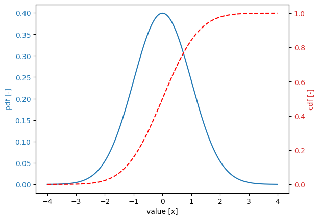
Let’s consider a normal distribution function with a location of 0.0 and a scale of 1.0:

stochast = Stochast()
stochast.distribution = DistributionType.normal
stochast.location = 0.0
stochast.scale = 1.0
stochast.plot()

To truncate a distribution, we use the truncated attribute.

stochast.truncated = True

The truncation interval is specified using the minimum and maximum properties. If these are not defined, the original domain of the distribution is used (i.e., no truncation is applied).

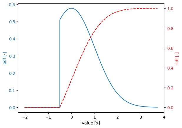
Suppose we want to truncate this distribution to the interval [-0.5, \infty). If this is the first time truncation is applied in the project, it is sufficient to specify only the minimum value:

stochast.minimum = -0.5

stochast.print()
stochast.plot()

Variable:
  distribution = normal (truncated)
Definition:
  location = 0.0
  scale = 1.0
  minimum = -0.5
  maximum = inf
Derived values:
  mean = 0.0
  deviation = 1.0
  variation = 0.0

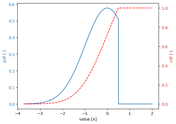
If we want to truncate the same distribution to the interval \((-\infty, 0.5]\), we need to specify both the minimum and maximum properties. Otherwise, the minimum would remain set to -0.5.

import numpy as np
stochast.truncated = True
stochast.minimum = -np.inf
stochast.maximum = 0.5

stochast.print()
stochast.plot()

Variable:
  distribution = normal (truncated)
Definition:
  location = 0.0
  scale = 1.0
  minimum = -inf
  maximum = 0.5
Derived values:
  mean = 0.0
  deviation = 1.0
  variation = 0.0

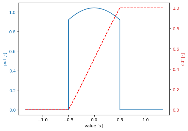
Below, we truncate the distribution to the interval \([-0.5, 0.5]\):

stochast.truncated = True
stochast.minimum = -0.5
stochast.maximum = 0.5

stochast.print()
stochast.plot()

Variable:
  distribution = normal (truncated)
Definition:
  location = 0.0
  scale = 1.0
  minimum = -0.5
  maximum = 0.5
Derived values:
  mean = 0.0
  deviation = 1.0
  variation = 0.0

Inverted distribution function

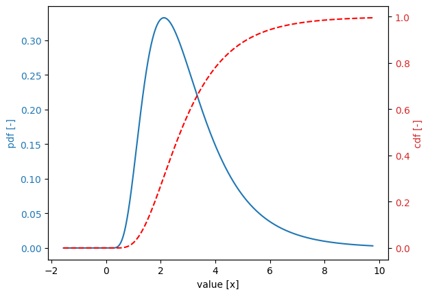
Let’s consider a log-normal distribution function with a locationof 1.0, a scale of 0.5 and a shift of 0.0:

stochast = Stochast()
stochast.distribution = DistributionType.log_normal
stochast.location = 1.0
stochast.scale = 0.5
stochast.shift = 0.0

stochast.print()
stochast.plot()

Variable:
  distribution = log_normal
Definition:
  location = 1.0
  scale = 0.5
  shift = 0.0
Derived values:
  mean = 3.080216848918031
  deviation = 1.6415718456238662
  variation = 0.5329403500277882

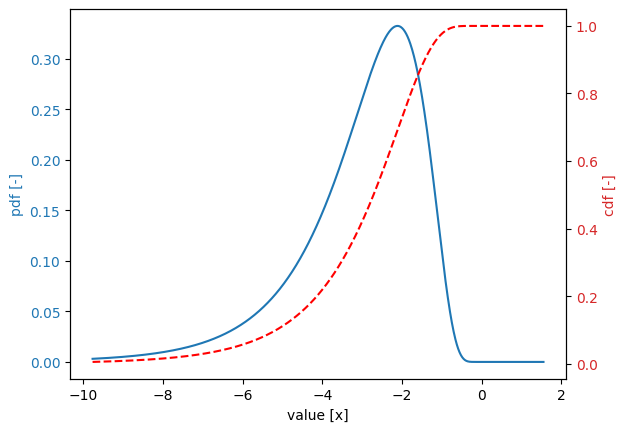
We want to invert this distribution function with respect to the shift value. This is done by setting the inverted attribute:

stochast.inverted = True

stochast.print()
stochast.plot()

Variable:
  distribution = log_normal (inverted)
Definition:
  location = 1.0
  scale = 0.5
  shift = 0.0
Derived values:
  mean = -3.080216848918031
  deviation = 1.6415718456238662
  variation = 0.5329403500277882

Fit parameters of a distribution function

It is also possible to estimate parameters of a distribution function from data. In this example, we consider the following dataset:

data = [2.3, 0.0, -1.0, 2.6, 2.7, 2.8, 3.3, 3.4, 1.0, 3.0, 0.0, -2.0, -1.0]

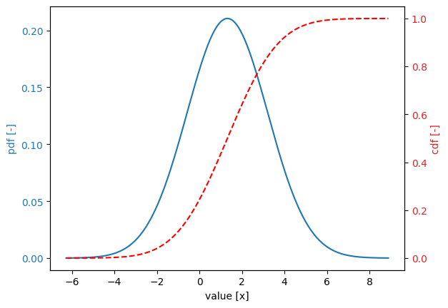
Let’s consider a normal distribution. By using stochast.fit(), we obtain the fitted location and scale:

stochast = Stochast()
stochast.distribution = DistributionType.normal
stochast.fit(data)

stochast.print()
stochast.plot()

Variable:
  distribution = normal
Definition:
  location = 1.3153846153846152
  scale = 1.8959809043720852
Derived values:
  mean = 1.3153846153846152
  deviation = 1.8959809043720852
  variation = 1.4413889916279012

The goodness of fit can be assessed using the Kolmogorov-Smirnov test through the get_ks_test() method:

def get_ks_test(data):
    print(f"kolmogorov smirnov test = {stochast.get_ks_test(data)}")

get_ks_test(data)

kolmogorov smirnov test = 0.23669173779063168

When we consider a log-normal distribution, the fitted parameters are as follows:

stochast = Stochast()
stochast.distribution = DistributionType.log_normal
stochast.fit(data)

stochast.print()
stochast.plot()

Variable:
  distribution = log_normal
Definition:
  location = 1.5964855623845133
  scale = 0.4261942592095209
  shift = -4.0
Derived values:
  mean = 1.4049020870683506
  deviation = 2.412211284018044
  variation = 1.7169960143284249

The result of the goodness-of-fit test is:

get_ks_test(data)

kolmogorov smirnov test = 0.2550238105742991