Sampling methods#

Estimation of failure probability due to wave run-up (Hunt’s equation)#

In this example, we will demonstrate the application of the sampling-based reliability methods (crude_monte_carlo, directional_sampling, importance_sampling, adaptive_importance_sampling, subset_simulation and latin_hypercube) to estimate the probability of failure of a levee due to wave run-up. The failure mechanism is characterized by the Hunt’s equation, which is a simple model to estimate the wave run-up.

Define model#

First, we import the necessary classes:

[27]:

from probabilistic_library import ReliabilityProject, DistributionType, ReliabilityMethod, SampleMethod

We consider the following limit state function:

$Z = h_{crest} - (h + R_u)$

where:

$h_{crest}$ is the crest height of the flood defence (m) $h$ is the water level on the flood defence (m) $R_u$ represents the wave run-up (m)

The wave run-up $R_u$ is derived using the Hunt’s equation:

$R_u = \xi \cdot H_s$

with:

$:nbsphinx-math:xi `= :nbsphinx-math:frac{tan (alpha)}{sqrt{2cdot pi cdot H_s/L_0}}` $

$L_0 = g \cdot T_p^2$

where:

$H_s$ is the significant wave height (m) $T_p$ is the peak wave period (s) $g$ is the gravitational acceleration ($9.81 m/s ^2$) $\tan (\alpha)$ is the slope of the flood defence (-)

The parameters $h$, $H_s$ and $T_p$ represent the imposed load, while $h_{crest}$ and $\tan (\alpha)$ stand for the strength of the levee.

[28]:

from utils.models import hunt

To perform a reliability analysis, we create a reliability project and specify the limit state function (model):

[29]:

project = ReliabilityProject()
project.model = hunt

project.model.print()

Model hunt:
Input parameters:
  t_p
  tan_alpha
  h_s
  h_crest
  h
Output parameters:
  Z

We assume the following distributions for the parameters present in the limit state function:

[30]:

project.variables["t_p"].distribution = DistributionType.log_normal
project.variables["t_p"].mean = 3
project.variables["t_p"].deviation = 1

project.variables["tan_alpha"].distribution = DistributionType.deterministic
project.variables["tan_alpha"].mean = 0.333333

project.variables["h_s"].distribution = DistributionType.log_normal
project.variables["h_s"].mean = 3
project.variables["h_s"].deviation = 1

project.variables["h_crest"].distribution = DistributionType.log_normal
project.variables["h_crest"].mean = 10
project.variables["h_crest"].deviation = 0.05

project.variables["h"].distribution = DistributionType.exponential
project.variables["h"].shift = 0.5
project.variables["h"].scale = 1

Perform reliability calculations with Crude Monte Carlo#

We start with the reliability method crude_monte_carlo. The reliability analysis is executed using project.run(), and the results are accessed from project.design_point.

[ ]:

project.settings.reliability_method = ReliabilityMethod.crude_monte_carlo
project.settings.minimum_samples = 10000
project.settings.maximum_samples = 50000
project.settings.variation_coefficient = 0.025
project.settings.save_realizations = True
project.settings.save_convergence = True

project.run()

project.design_point.print()
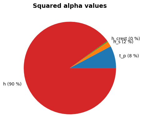
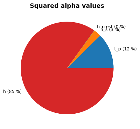
project.design_point.plot_alphas()
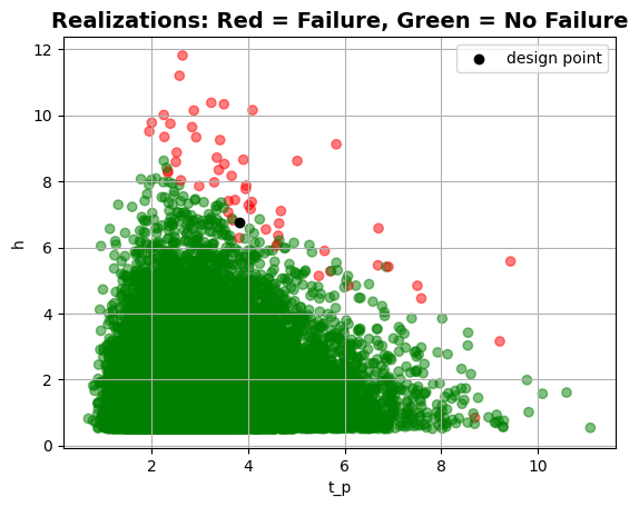
project.design_point.plot_realizations()
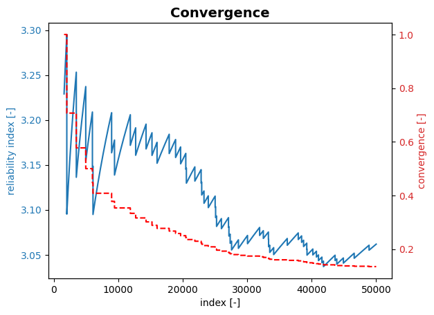
project.design_point.plot_convergence()

Reliability:
 Reliability index = 3.062
 Probability of failure = 0.0011
 Convergence = 0.1348 (not converged)
 Model runs = 50001
Alpha values:
 t_p: alpha = -0.299, x = 3.831
 tan_alpha: alpha = 0, x = 0.3333
 h_s: alpha = -0.1287, x = 3.234
 h_crest: alpha = -0.04707, x = 10.01
 h: alpha = -0.9444, x = 6.757

../_images/_examples_reliability_methods_hunt_9_1.png

../_images/_examples_reliability_methods_hunt_9_2.png

../_images/_examples_reliability_methods_hunt_9_3.png

Perform reliability calculations with Directional Sampling#

We now conduct the reliability analysis using the directional_sampling method.

[32]:

project.settings.reliability_method = ReliabilityMethod.directional_sampling
project.settings.minimum_directions = 10000
project.settings.maximum_directions = 20000
project.settings.variation_coefficient = 0.02

project.run()

project.design_point.print()
project.design_point.plot_alphas()

Reliability (Directional Sampling)
 Reliability index = 3.068
 Probability of failure = 0.001078
 Convergence = 0.02748 (not converged)
 Model runs = 111509
Alpha values:
 t_p: alpha = -0.3346, x = 3.972
 tan_alpha: alpha = 0, x = 0.3333
 h_s: alpha = -0.1756, x = 3.39
 h_crest: alpha = 0.006802, x = 9.999
 h: alpha = -0.9258, x = 6.595

../_images/_examples_reliability_methods_hunt_11_1.png

Perform reliability calculations with Importance Sampling#

We now conduct the reliability analysis using the importance_sampling assuming the start value of $u=1$ for the three random variables:

[33]:

project.settings.reliability_method = ReliabilityMethod.importance_sampling
project.settings.minimum_samples = 1000
project.settings.maximum_samples = 100000
project.settings.variation_coefficient = 0.02

project.settings.stochast_settings["t_p"].start_value = 1
project.settings.stochast_settings["h_s"].start_value = 1
project.settings.stochast_settings["h"].start_value = 1

project.run()

project.design_point.print()
project.design_point.plot_alphas()

#reset values
project.settings.stochast_settings["t_p"].start_value = 0
project.settings.stochast_settings["h_s"].start_value = 0
project.settings.stochast_settings["h"].start_value = 0

Reliability:
 Reliability index = 3.072
 Probability of failure = 0.001063
 Convergence = 0.02342 (not converged)
 Model runs = 100001
Alpha values:
 t_p: alpha = -0.3346, x = 3.973
 tan_alpha: alpha = 0, x = 0.3333
 h_s: alpha = -0.1721, x = 3.379
 h_crest: alpha = 0.009329, x = 9.998
 h: alpha = -0.9265, x = 6.613

../_images/_examples_reliability_methods_hunt_13_1.png

Perform reliability calculations with Adaptive Importance Sampling#

We now conduct the reliability analysis using the adaptive_importance_sampling method.

[34]:

project.settings.reliability_method = ReliabilityMethod.adaptive_importance_sampling
project.settings.minimum_samples = 10000
project.settings.maximum_samples = 100000
project.settings.minimum_variance_loops = 5
project.settings.maximum_variance_loops = 10
project.settings.fraction_failed = 0.5
project.settings.variation_coefficient = 0.02

project.run()

project.design_point.print()
project.design_point.plot_alphas()

Reliability:
 Reliability index = 3.069
 Probability of failure = 0.001072
 Convergence = 0.02 (converged)
 Model runs = 50976
Alpha values:
 t_p: alpha = -0.3317, x = 3.961
 tan_alpha: alpha = 0, x = 0.3333
 h_s: alpha = -0.1642, x = 3.352
 h_crest: alpha = 0.01283, x = 9.998
 h: alpha = -0.9289, x = 6.63

Contributing design points:
  Reliability (Variance loop 1)
   Reliability index = 3.074
   Probability of failure = 0.001057
   Convergence = 0.1529 (not converged)
   Model runs = 10001
  Alpha values:
   t_p: alpha = -0.3606, x = 4.079
   tan_alpha: alpha = 0, x = 0.3333
   h_s: alpha = -0.2178, x = 3.537
   h_crest: alpha = -0.02189, x = 10
   h: alpha = -0.9066, x = 6.429

  Reliability (Variance loop 2)
   Reliability index = 3.07
   Probability of failure = 0.001069
   Convergence = 0.04657 (not converged)
   Model runs = 10001
  Alpha values:
   t_p: alpha = -0.3252, x = 3.935
   tan_alpha: alpha = 0, x = 0.3333
   h_s: alpha = -0.1697, x = 3.37
   h_crest: alpha = 0.01776, x = 9.997
   h: alpha = -0.9301, x = 6.644

  Reliability (Variance loop 3)
   Reliability index = 3.066
   Probability of failure = 0.001084
   Convergence = 0.04522 (not converged)
   Model runs = 10001
  Alpha values:
   t_p: alpha = -0.3276, x = 3.943
   tan_alpha: alpha = 0, x = 0.3333
   h_s: alpha = -0.1658, x = 3.357
   h_crest: alpha = 0.01809, x = 9.997
   h: alpha = -0.93, x = 6.63

  Reliability (Variance loop 4)
   Reliability index = 3.065
   Probability of failure = 0.001089
   Convergence = 0.04522 (not converged)
   Model runs = 10001
  Alpha values:
   t_p: alpha = -0.3279, x = 3.944
   tan_alpha: alpha = 0, x = 0.3333
   h_s: alpha = -0.1646, x = 3.352
   h_crest: alpha = 0.01749, x = 9.997
   h: alpha = -0.9301, x = 6.628

  Reliability (Variance loop 5)
   Reliability index = 3.065
   Probability of failure = 0.001087
   Convergence = 0.04526 (not converged)
   Model runs = 10001
  Alpha values:
   t_p: alpha = -0.3273, x = 3.942
   tan_alpha: alpha = 0, x = 0.3333
   h_s: alpha = -0.1649, x = 3.353
   h_crest: alpha = 0.0173, x = 9.997
   h: alpha = -0.9303, x = 6.631

  Reliability (Variance loop 6)
   Reliability index = 3.065
   Probability of failure = 0.001089
   Convergence = 0.04525 (not converged)
   Model runs = 10001
  Alpha values:
   t_p: alpha = -0.3276, x = 3.943
   tan_alpha: alpha = 0, x = 0.3333
   h_s: alpha = -0.1647, x = 3.353
   h_crest: alpha = 0.01697, x = 9.997
   h: alpha = -0.9302, x = 6.628

  Reliability (Variance loop 7)
   Reliability index = 3.065
   Probability of failure = 0.001088
   Convergence = 0.04527 (not converged)
   Model runs = 10001
  Alpha values:
   t_p: alpha = -0.3276, x = 3.943
   tan_alpha: alpha = 0, x = 0.3333
   h_s: alpha = -0.1649, x = 3.354
   h_crest: alpha = 0.01729, x = 9.997
   h: alpha = -0.9302, x = 6.629

  Reliability (Variance loop 8)
   Reliability index = 3.064
   Probability of failure = 0.00109
   Convergence = 0.04524 (not converged)
   Model runs = 10001
  Alpha values:
   t_p: alpha = -0.3274, x = 3.942
   tan_alpha: alpha = 0, x = 0.3333
   h_s: alpha = -0.1646, x = 3.352
   h_crest: alpha = 0.01697, x = 9.997
   h: alpha = -0.9303, x = 6.628

  Reliability (Variance loop 9)
   Reliability index = 3.065
   Probability of failure = 0.001087
   Convergence = 0.04529 (not converged)
   Model runs = 10001
  Alpha values:
   t_p: alpha = -0.3273, x = 3.942
   tan_alpha: alpha = 0, x = 0.3333
   h_s: alpha = -0.1654, x = 3.355
   h_crest: alpha = 0.01726, x = 9.997
   h: alpha = -0.9302, x = 6.629

../_images/_examples_reliability_methods_hunt_15_1.png

Perform reliability calculations with Subset Simulation#

We now conduct the reliability analysis using the subset_simulation method.

[35]:

project.settings.reliability_method = ReliabilityMethod.subset_simulation
project.settings.minimum_samples = 1000
project.settings.maximum_samples = 50000
project.settings.variation_coefficient = 0.02
project.settings.sample_method = SampleMethod.adaptive_conditional

project.run()

project.design_point.print()
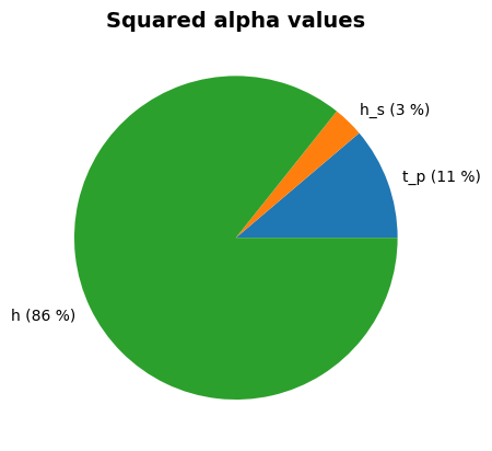
project.design_point.plot_alphas()

Reliability:
 Reliability index = 3.077
 Probability of failure = 0.001047
 Convergence = 0.01308 (not converged)
 Model runs = 45000
Alpha values:
 t_p: alpha = -0.3517, x = 4.044
 tan_alpha: alpha = 0, x = 0.3333
 h_s: alpha = -0.1625, x = 3.348
 h_crest: alpha = 0.02568, x = 9.996
 h: alpha = -0.9215, x = 6.579

Contributing design points:
  Reliability (Subset iteration 1)
   Reliability index = 3.062
   Probability of failure = 0.0011
   Convergence = 0.1348 (not converged)
   Model runs = 50001
  Alpha values:
   t_p: alpha = -0.299, x = 3.831
   tan_alpha: alpha = 0, x = 0.3333
   h_s: alpha = -0.1287, x = 3.234
   h_crest: alpha = -0.04707, x = 10.01
   h: alpha = -0.9444, x = 6.757

  Reliability (Subset iteration 2)
   Reliability index = 3.075
   Probability of failure = 0.001054
   Convergence = 0.04333 (not converged)
   Model runs = 45000
  Alpha values:
   t_p: alpha = -0.3562, x = 4.061
   tan_alpha: alpha = 0, x = 0.3333
   h_s: alpha = -0.1712, x = 3.376
   h_crest: alpha = 0.01876, x = 9.997
   h: alpha = -0.9184, x = 6.543

../_images/_examples_reliability_methods_hunt_17_1.png

Perform reliability calculations with Latin hypercube#

We now conduct the reliability analysis using the latin_hypercube.

[36]:

project.settings.reliability_method = ReliabilityMethod.latin_hypercube
project.settings.minimum_samples = 100000

project.run()

project.design_point.print()
project.design_point.plot_alphas()

Reliability:
 Reliability index = 3.076
 Probability of failure = 0.00105
 Convergence = 0.09754 (not converged)
 Model runs = 100001
Alpha values:
 t_p: alpha = -0.2787, x = 3.759
 tan_alpha: alpha = 0, x = 0.3333
 h_s: alpha = -0.1373, x = 3.264
 h_crest: alpha = 0.05574, x = 9.991
 h: alpha = -0.9489, x = 6.843

../_images/_examples_reliability_methods_hunt_19_1.png