Numerical methods#
Estimation of piping failure probability (Bligh’s model)#
In this example, we will demonstrate the application of the numerical reliability methods (numerical_integration and numerical_bisection) to estimate the probability of failure of a levee due to piping mechanism. The failure mechanism is characterized here using the simple model of Bligh.
Define model#
First, we import the necessary classes:
[8]:
from probabilistic_library import ReliabilityProject, DistributionType, ReliabilityMethod
The limit state function according to the piping model of Bligh is defined as follows:
\(Z = \frac{m \cdot L}{c_{creep}} -\Delta H\)
where:
\(\Delta H\) is the difference between the water level on the levee and the water level in the polder (m) \(L\) is the seepage path length (m) \(m\) represents model uncertainty (-) \(c_{creep}\) is the creep factor (-)
The parameter \(\Delta H\) represents the imposed load, while \(L\) stands for the strength of the levee. The creep factor value for very fine-grained sand is \(18\).
[9]:
from utils.models import bligh
To perform a reliability analysis, we create a reliability project and specify the limit state function (model):
[10]:
project = ReliabilityProject()
project.model = bligh

project.model.print()
Model bligh:
Input parameters:
  m
  L
  c_creep
  delta_H
Output parameters:
  Z
We assume the following distributions for the parameters \(m\), \(L\), \(c_{creep}\) and \(\Delta H\):
[11]:
project.variables["m"].distribution = DistributionType.log_normal
project.variables["m"].mean = 1.76
project.variables['m'].deviation = 1.69

project.variables["L"].distribution = DistributionType.normal
project.variables["L"].mean = 50
project.variables["L"].deviation = 2.5

project.variables["c_creep"].distribution = DistributionType.deterministic
project.variables["c_creep"].mean = 18

project.variables["delta_H"].distribution = DistributionType.gumbel
project.variables["delta_H"].shift = 0.53
project.variables["delta_H"].scale = 0.406
Perform reliability calculations with Numerical Integration#
We start with the reliability method numerical_integration. The reliability analysis is executed using project.run(), and the results are accessed from project.design_point.
[12]:
project.settings.reliability_method = ReliabilityMethod.numerical_integration
project.settings.stochast_settings["m"].intervals = 50
project.settings.stochast_settings["L"].intervals = 20
project.settings.stochast_settings["delta_H"].intervals = 50
project.settings.save_realizations = True
project.run()
project.design_point.print()
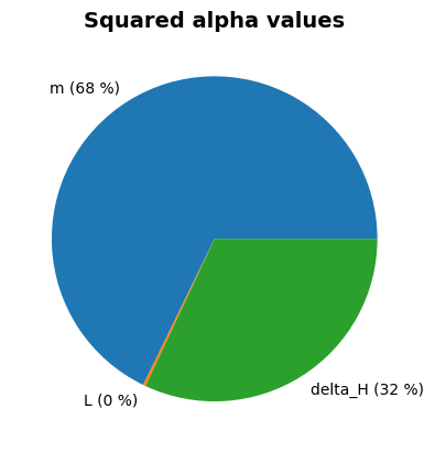
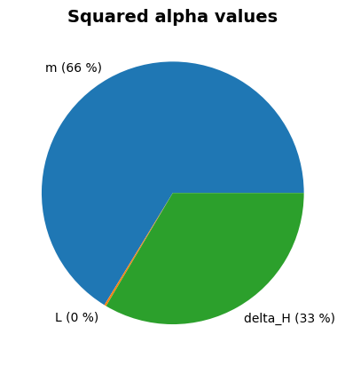
project.design_point.plot_alphas()
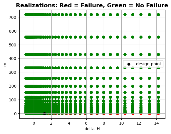
project.design_point.plot_realizations()
Reliability:
 Reliability index = 1.661
 Probability of failure = 0.0484
 Model runs = 50001
Alpha values:
 m: alpha = 0.8141, x = 0.4257
 L: alpha = 0.04915, x = 49.8
 c_creep: alpha = 0, x = 18
 delta_H: alpha = -0.5787, x = 1.217
Perform reliability calculations with Numerical bisection#
We now conduct the reliability analysis using the numerical_bisection method.
[13]:
project.settings.reliability_method = ReliabilityMethod.numerical_bisection
project.settings.minimum_iterations = 5
project.settings.maximum_iterations = 10
project.settings.epsilon_beta = 0.1
project.run()
project.design_point.print()
project.design_point.plot_alphas()
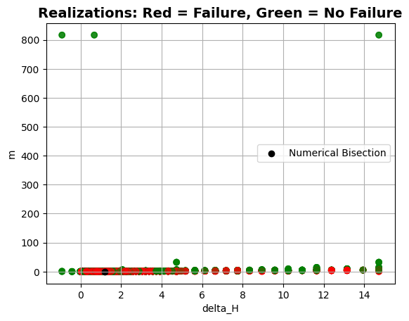
project.design_point.plot_realizations()
Reliability (Numerical Bisection)
 Reliability index = 1.66
 Probability of failure = 0.04851
 Convergence = 0.09003 (not converged)
 Model runs = 10343
Alpha values:
 m: alpha = 0.8233, x = 0.4207
 L: alpha = 0.05128, x = 49.79
 c_creep: alpha = 0, x = 18
 delta_H: alpha = -0.5653, x = 1.202