System reliability analysis

In this example, we will demonstrate how to perform a reliability analysis of a system consisting of two components. We will analyze two system configurations:

• Parallel System: the system fails only when both components fail.

• Series System: the system fails when at least one of the components fails.

Define Limit State Functions

First, we import the necessary classes:

from probabilistic_library import ReliabilityProject, ReliabilityMethod, DistributionType, CombineProject, CombinerMethod, CombineType, Stochast

We consider two elements, each described by the following limit state functions:

\(Z_1 = 1.9 - (a+b)\)

\(Z_2 = 1.85 - (1.5 \cdot b + 0.5 \cdot c)\)

from utils.models import linear_a_b, linear_b_c

Note that both functions share a common variable \(b\).

We consider two system configurations:

• Parallel system: the system fails only when both \(Z_1\) and \(Z_2\) are less than zero.

• Series system: the system fails when either \(Z_1\) or \(Z_2\) is less than zero.

In the first case we want to calculate the probability \(P(Z_1<0 \cap Z_2<0)\) and, in the second case, the probability \(P(Z_1<0 \cup Z_2<0)\).

Perform reliability calculations for each element

First, we perform the reliability analysis of the individual elements (described by the limit state functions).

We create a reliability project ReliabilityProject(). We assume that variables \(a\) and \(b\) are uniformly distributed over the interval \([-1, 1]\). The variable \(c\) is normally distributed with a mean of \(0.1\) and a deviation of \(0.8\). We use the First Order Reliability Method (FORM) to run the reliability analysis.

It is essential to define the limit state function model before specifying the random variables!

Using project.run() we execute the reliability analysis for one limit state function. The results are stored in project.design_point. To combine the results later, we store the outputs in separate objects (dp_Z1 and dp_Z2).

project = ReliabilityProject()
project.settings.reliability_method = ReliabilityMethod.form
project.settings.relaxation_factor = 0.75
project.settings.maximum_iterations = 50
project.settings.epsilon_beta = 0.01

project.model = linear_a_b

project.variables["a"].distribution = DistributionType.uniform
project.variables["a"].minimum = -1
project.variables["a"].maximum = 1

project.variables["b"].distribution = DistributionType.uniform
project.variables["b"].minimum = -1
project.variables["b"].maximum = 1

project.run()
dp_Z1 = project.design_point
dp_Z1.identifier = "Z1"
dp_Z1.print()

project.model = linear_b_c

project.variables["c"].distribution = DistributionType.normal
project.variables["c"].mean = 0.1
project.variables["c"].deviation = 0.8

project.run()
dp_Z2 = project.design_point
dp_Z2.identifier = "Z2"
dp_Z2.print()

Reliability (Z1)
 Reliability index = 2.772
 Probability of failure = 0.002783
 Convergence = 0.004051 (converged)
 Model runs = 21
Alpha values:
 a: alpha = -0.7071, x = 0.95
 b: alpha = -0.7071, x = 0.95

Reliability (Z2)
 Reliability index = 1.95
 Probability of failure = 0.02559
 Convergence = 0.007929 (converged)
 Model runs = 18
Alpha values:
 b: alpha = -0.719, x = 0.8391
 c: alpha = -0.695, x = 1.184

Perform reliability analysis of a system

To perform the reliability analysis of a system, we create a new project using CombineProject(). We append the reliability results of the individual elements to this object.

combine_project = CombineProject()

combine_project.design_points.append(dp_Z1)
combine_project.design_points.append(dp_Z2)

The library offers the following methods for the reliability analysis of a system: hohenbichler, hohenbichler_form, importance_sampling, directional_sampling. The desired reliability method can be set using combine_project.settings.combiner_method.

The type of system configuration (series or parallel) can be defined using combine_project.combine_type.

Execute the reliability analysis of the system using combine_project.run(). The results will be stored in combine_project.design_point.

def fault_tree(combine_project, combine_type):

    combine_algorithms = [CombinerMethod.hohenbichler, CombinerMethod.hohenbichler_form, CombinerMethod.importance_sampling, CombinerMethod.directional_sampling]

    combine_project.settings.combine_type = combine_type
    combine_algorithms = [CombinerMethod.hohenbichler, CombinerMethod.importance_sampling, CombinerMethod.directional_sampling]

    for combine_algorithm in combine_algorithms:

        combine_project.settings.combiner_method = combine_algorithm
        combine_project.run()
        dp = combine_project.design_point
        dp.identifier = str(combine_type) + ' - ' + str(combine_algorithm)

        dp.print()

fault_tree(combine_project, CombineType.series)
fault_tree(combine_project, CombineType.parallel)

Reliability (series - hohenbichler)
 Reliability index = 1.92
 Probability of failure = 0.02746
 Model runs = 0
Alpha values:
 a: alpha = -0.0725, x = 0.95
 b: alpha = -0.7507, x = 0.95
 c: alpha = -0.6567, x = 0

Contributing design points:
  Reliability (Z1)
   Reliability index = 2.772
   Probability of failure = 0.002783
   Convergence = 0.004051 (converged)
   Model runs = 21
  Alpha values:
   a: alpha = -0.7071, x = 0.95
   b: alpha = -0.7071, x = 0.95

  Reliability (Z2)
   Reliability index = 1.95
   Probability of failure = 0.02559
   Convergence = 0.007929 (converged)
   Model runs = 18
  Alpha values:
   b: alpha = -0.719, x = 0.8391
   c: alpha = -0.695, x = 1.184

Reliability (series - importance_sampling)
 Reliability index = 1.919
 Probability of failure = 0.02749
 Model runs = 0
Alpha values:
 a: alpha = -0.1006, x = 0.1531
 b: alpha = -0.7622, x = 0.8564
 c: alpha = -0.6395, x = 1.082

Contributing design points:
  Reliability (Z2)
   Reliability index = 1.95
   Probability of failure = 0.02559
   Convergence = 0.007929 (converged)
   Model runs = 18
  Alpha values:
   b: alpha = -0.719, x = 0.8391
   c: alpha = -0.695, x = 1.184

  Reliability (Z1)
   Reliability index = 2.772
   Probability of failure = 0.002783
   Convergence = 0.004051 (converged)
   Model runs = 21
  Alpha values:
   a: alpha = -0.7071, x = 0.95
   b: alpha = -0.7071, x = 0.95

Reliability (series - directional_sampling)
 Reliability index = 1.998
 Probability of failure = 0.02288
 Convergence = 0.07704 (converged)
 Model runs = 1
Alpha values:
 a: alpha = -0.08834, x = 0.1401
 b: alpha = -0.7648, x = 0.8734
 c: alpha = -0.6382, x = 1.12

Contributing design points:
  Reliability (Z1)
   Reliability index = 2.772
   Probability of failure = 0.002783
   Convergence = 0.004051 (converged)
   Model runs = 21
  Alpha values:
   a: alpha = -0.7071, x = 0.95
   b: alpha = -0.7071, x = 0.95

  Reliability (Z2)
   Reliability index = 1.95
   Probability of failure = 0.02559
   Convergence = 0.007929 (converged)
   Model runs = 18
  Alpha values:
   b: alpha = -0.719, x = 0.8391
   c: alpha = -0.695, x = 1.184

Reliability (parallel - hohenbichler)
 Reliability index = 3.117
 Probability of failure = 0.0009126
 Model runs = 0
Alpha values:
 a: alpha = -0.5306, x = 0.95
 b: alpha = -0.8053, x = 0.95
 c: alpha = -0.2645, x = 0

Contributing design points:
  Reliability (Z1)
   Reliability index = 2.772
   Probability of failure = 0.002783
   Convergence = 0.004051 (converged)
   Model runs = 21
  Alpha values:
   a: alpha = -0.7071, x = 0.95
   b: alpha = -0.7071, x = 0.95

  Reliability (Z2)
   Reliability index = 1.95
   Probability of failure = 0.02559
   Convergence = 0.007929 (converged)
   Model runs = 18
  Alpha values:
   b: alpha = -0.719, x = 0.8391
   c: alpha = -0.695, x = 1.184

Reliability (parallel - importance_sampling)
 Reliability index = 3.123
 Probability of failure = 0.000894
 Convergence = 0.01692 (converged)
 Model runs = 21000
Alpha values:
 a: alpha = -0.5401, x = 0.9084
 b: alpha = -0.7988, x = 0.9874
 c: alpha = -0.2649, x = 0.7618

Contributing design points:
  Reliability (Z1)
   Reliability index = 2.772
   Probability of failure = 0.002783
   Convergence = 0.004051 (converged)
   Model runs = 21
  Alpha values:
   a: alpha = -0.7071, x = 0.95
   b: alpha = -0.7071, x = 0.95

  Reliability (Z2)
   Reliability index = 1.95
   Probability of failure = 0.02559
   Convergence = 0.007929 (converged)
   Model runs = 18
  Alpha values:
   b: alpha = -0.719, x = 0.8391
   c: alpha = -0.695, x = 1.184

Reliability (parallel - directional_sampling)
 Reliability index = 3.144
 Probability of failure = 0.0008344
 Convergence = 0.09989 (converged)
 Model runs = 1
Alpha values:
 a: alpha = -0.5342, x = 0.9069
 b: alpha = -0.7906, x = 0.9871
 c: alpha = -0.2993, x = 0.8527

Contributing design points:
  Reliability (Z1)
   Reliability index = 2.772
   Probability of failure = 0.002783
   Convergence = 0.004051 (converged)
   Model runs = 21
  Alpha values:
   a: alpha = -0.7071, x = 0.95
   b: alpha = -0.7071, x = 0.95

  Reliability (Z2)
   Reliability index = 1.95
   Probability of failure = 0.02559
   Convergence = 0.007929 (converged)
   Model runs = 18
  Alpha values:
   b: alpha = -0.719, x = 0.8391
   c: alpha = -0.695, x = 1.184

Uncorrelated \(b\) variable

In the previous calculations, the variable \(b\) in the limit state function \(Z_1\)​ was assumed to be the same as the variable \(b\) in the limit state function \(Z_2\)​, implying a perfect correlation (correlation coefficient of \(1.0\)). This section demonstrates the impact of this assumption on the reliability analysis results.

To explore the effect of relaxing this assumption, we will now assume that the variable \(b\) in \(Z_1\) is not correlated with the variable \(b\) in \(Z_2\). Specifically, we set the correlation coefficient to \(0.0\).

combine_project.correlation_matrix["b"] = 0.0

fault_tree(combine_project, CombineType.series)
fault_tree(combine_project, CombineType.parallel)

Reliability (series - hohenbichler)
 Reliability index = 1.906
 Probability of failure = 0.0283
 Model runs = 0
Alpha values:
 a: alpha = -0.09896, x = 0.95
 b: alpha = -0.7188, x = 0.95
 c: alpha = -0.6882, x = 0

Contributing design points:
  Reliability (Z1)
   Reliability index = 2.772
   Probability of failure = 0.002783
   Convergence = 0.004051 (converged)
   Model runs = 21
  Alpha values:
   a: alpha = -0.7071, x = 0.95
   b: alpha = -0.7071, x = 0.95

  Reliability (Z2)
   Reliability index = 1.95
   Probability of failure = 0.02559
   Convergence = 0.007929 (converged)
   Model runs = 18
  Alpha values:
   b: alpha = -0.719, x = 0.8391
   c: alpha = -0.695, x = 1.184

Reliability (series - importance_sampling)
 Reliability index = 1.907
 Probability of failure = 0.02827
 Model runs = 0
Alpha values:
 a: alpha = -0.1006, x = 0.1521
 b: alpha = -0.7622, x = 0.8539
 c: alpha = -0.6395, x = 1.076

Contributing design points:
  Reliability (Z2)
   Reliability index = 1.95
   Probability of failure = 0.02559
   Convergence = 0.007929 (converged)
   Model runs = 18
  Alpha values:
   b: alpha = -0.719, x = 0.8391
   c: alpha = -0.695, x = 1.184

  Reliability (Z1)
   Reliability index = 2.772
   Probability of failure = 0.002783
   Convergence = 0.004051 (converged)
   Model runs = 21
  Alpha values:
   a: alpha = -0.7071, x = 0.95
   b: alpha = -0.7071, x = 0.95

Reliability (series - directional_sampling)
 Reliability index = 1.901
 Probability of failure = 0.02866
 Convergence = 0.08284 (converged)
 Model runs = 1
Alpha values:
 a: alpha = -0.09078, x = 0.137
 b: alpha = -0.7452, x = 0.8434
 c: alpha = -0.6607, x = 1.105

Contributing design points:
  Reliability (Z1)
   Reliability index = 2.772
   Probability of failure = 0.002783
   Convergence = 0.004051 (converged)
   Model runs = 21
  Alpha values:
   a: alpha = -0.7071, x = 0.95
   b: alpha = -0.7071, x = 0.95

  Reliability (Z2)
   Reliability index = 1.95
   Probability of failure = 0.02559
   Convergence = 0.007929 (converged)
   Model runs = 18
  Alpha values:
   b: alpha = -0.719, x = 0.8391
   c: alpha = -0.695, x = 1.184

Reliability (parallel - hohenbichler)
 Reliability index = 3.804
 Probability of failure = 7.12e-05
 Model runs = 0
Alpha values:
 a: alpha = -0.5636, x = 0.95
 b: alpha = -0.7115, x = 0.95
 c: alpha = -0.4197, x = 0

Contributing design points:
  Reliability (Z1)
   Reliability index = 2.772
   Probability of failure = 0.002783
   Convergence = 0.004051 (converged)
   Model runs = 21
  Alpha values:
   a: alpha = -0.7071, x = 0.95
   b: alpha = -0.7071, x = 0.95

  Reliability (Z2)
   Reliability index = 1.95
   Probability of failure = 0.02559
   Convergence = 0.007929 (converged)
   Model runs = 18
  Alpha values:
   b: alpha = -0.719, x = 0.8391
   c: alpha = -0.695, x = 1.184

Reliability (parallel - importance_sampling)
 Reliability index = 3.799
 Probability of failure = 7.254e-05
 Convergence = 0.0349 (converged)
 Model runs = 21000
Alpha values:
 a: alpha = -0.556, x = 0.9653
 b: alpha = -0.7186, x = 0.9937
 c: alpha = -0.4177, x = 1.37

Contributing design points:
  Reliability (Z1)
   Reliability index = 2.772
   Probability of failure = 0.002783
   Convergence = 0.004051 (converged)
   Model runs = 21
  Alpha values:
   a: alpha = -0.7071, x = 0.95
   b: alpha = -0.7071, x = 0.95

  Reliability (Z2)
   Reliability index = 1.95
   Probability of failure = 0.02559
   Convergence = 0.007929 (converged)
   Model runs = 18
  Alpha values:
   b: alpha = -0.719, x = 0.8391
   c: alpha = -0.695, x = 1.184

Reliability (parallel - directional_sampling)
 Reliability index = 3.745
 Probability of failure = 9.029e-05
 Convergence = 0.09981 (converged)
 Model runs = 1
Alpha values:
 a: alpha = -0.5543, x = 0.9621
 b: alpha = -0.7198, x = 0.993
 c: alpha = -0.4179, x = 1.352

Contributing design points:
  Reliability (Z1)
   Reliability index = 2.772
   Probability of failure = 0.002783
   Convergence = 0.004051 (converged)
   Model runs = 21
  Alpha values:
   a: alpha = -0.7071, x = 0.95
   b: alpha = -0.7071, x = 0.95

  Reliability (Z2)
   Reliability index = 1.95
   Probability of failure = 0.02559
   Convergence = 0.007929 (converged)
   Model runs = 18
  Alpha values:
   b: alpha = -0.719, x = 0.8391
   c: alpha = -0.695, x = 1.184

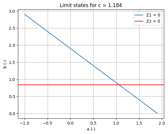
Additionally, let’s plot the limit state functions (\(Z = 0\)):

import matplotlib.pyplot as plt
import numpy as np

def linear_a_b_zero(a):
    b = 1.9 - a
    return b

def linear_b_c_zero(c):
    b = (1.85 - 0.5 * c) / 1.5
    return b

a = np.arange(-1.0, 2.0, 0.1)
c = [1.184]

b_z1 = [linear_a_b_zero(val) for val in a]
b_z2 = [linear_b_c_zero(val) for val in c]

plt.plot(a, b_z1, label='Z1 = 0')
plt.axhline(y=b_z2, color='r', label='Z2 = 0')
plt.grid()
plt.legend()
plt.xlabel('a (-)')
plt.ylabel('b (-)')
plt.title(f'Limit states for c = {c[0]}')
plt.show()