Fragility curves

Failure probability calculations with a fragility curve

In this example, we will demonstrate how to calculate the failure probability of a levee using a fragility curve.

Fragility curve is a function that describes the relation between the load imposed on the levee and the corresponding (conditional) failure probability. Typically a fragility curve is expressed by the following relation: \(h \rightarrow P(Z<0|h)\). By integrating the fragility curve with the load statistics, the failure probability can be estimated. The goal is to derive the following probability:

\(P(Z<0) = \int P(Z<0 | h)\cdot f(h) dh\)

First, let’s import the necessary packages:

from probabilistic_library import ReliabilityProject, DistributionType, ReliabilityMethod, FragilityCurve, FragilityValue, Stochast
import matplotlib.pyplot as plt
import numpy as np

We consider the Hunt’s limit state function:

from utils.models import hunt

We define a reliability project using the ReliabilityProject() class and refer to the Hunt’s limit state function:

project = ReliabilityProject()
project.model = hunt

project.model.print()

Model hunt:
Input parameters:
  t_p
  tan_alpha
  h_s
  h_crest
  h
Output parameters:
  Z

We define the associated variables, except for the water level variable, \(h\):

project.variables["t_p"].distribution = DistributionType.log_normal
project.variables["t_p"].mean = 6
project.variables["t_p"].deviation = 2

project.variables["tan_alpha"].distribution = DistributionType.deterministic
project.variables["tan_alpha"].mean = 0.333333

project.variables["h_s"].distribution = DistributionType.log_normal
project.variables["h_s"].mean = 3
project.variables["h_s"].deviation = 1

project.variables["h_crest"].distribution = DistributionType.log_normal
project.variables["h_crest"].mean = 10
project.variables["h_crest"].deviation = 0.05

We choose the form calculation method:

project.settings.reliability_method = ReliabilityMethod.form
project.settings.relaxation_factor = 0.15
project.settings.maximum_iterations = 50
project.settings.epsilon_beta = 0.01

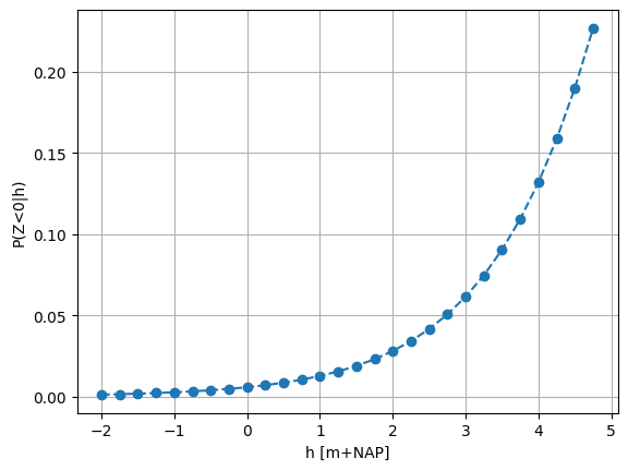
Next, we construct the fragility curve using the FragilityCurve() class, providing the water level variable \(h\). Reliability calculations are performed for each value of the water level variable.

fragility_curve = FragilityCurve()
fragility_curve.name = "conditional"

fc_pf = []
h = np.arange(-2.0, 5.0, 0.25)
for val in h:

        project.variables["h"].distribution = DistributionType.deterministic
        project.variables["h"].mean = val
        project.run()
        dp = project.design_point

        value = FragilityValue()
        value.x = val
        value.reliability_index = dp.reliability_index
        value.design_point = dp

        fragility_curve.fragility_values.append(value)
        fc_pf.append(dp.probability_failure)

The calculations above result in a fragility curve:

plt.plot(h, fc_pf, 'o--')
plt.grid()
plt.xlabel("h [m+NAP]")
plt.ylabel("P(Z<0|h)")
plt.show()

The load \(h\) is the integrand and follows an exponential distribution:

integrand = Stochast()
integrand.name = "h"
integrand.distribution = DistributionType.exponential
integrand.shift = 0.5
integrand.scale = 1.0

The integration of the fragility curve with the water level statistics is performed as follows:

dp = fragility_curve.integrate(integrand)

The results are:

dp.print()

Reliability:
 Reliability index = 1.8853
 Probability of failure = 0.0297
 Convergence = 0.0 (converged)
 Model runs = 16001
Alpha values:
 h: alpha = -0.5209, x = 2.3137
 t_p: alpha = -0.8555, x = 9.6084
 h_s: alpha = -0.4226, x = 3.6859
 h_crest: alpha = 0.0168, x = 9.9983

Reliability calculations performed without the fragility curve, but instead using the distribution function for the water level \(h\), should yield results that are close to those obtained using the fragility curve.

We begin with the form method, which provides a reliability index that deviates from the one obtained from the integration of the water level distribution with the fragility curve. It is expected that the method has converged to a local optimum in this case.

project.variables["h"].distribution = DistributionType.exponential
project.variables["h"].shift = 0.5
project.variables["h"].scale = 1.0

project.run()

project.design_point.print()

Reliability (FORM)
 Reliability index = 2.0502
 Probability of failure = 0.0202
 Convergence = 0.0089 (converged)
 Model runs = 165
Alpha values:
 t_p: alpha = -0.7813, x = 9.5736
 tan_alpha: alpha = 0.0, x = 0.3333
 h_s: alpha = -0.3859, x = 3.6793
 h_crest: alpha = 0.0154, x = 9.9983
 h: alpha = -0.4904, x = 2.3491

The results are improved, when the crude_monte_carlo method is used:

project.settings.reliability_method = ReliabilityMethod.crude_monte_carlo
project.settings.minimum_samples = 1000
project.settings.maximum_samples = 50000
project.settings.variation_coefficient = 0.02

project.run()

project.design_point.print()

Reliability:
 Reliability index = 1.8832
 Probability of failure = 0.0298
 Convergence = 0.0255 (not converged)
 Model runs = 50001
Alpha values:
 t_p: alpha = -0.7713, x = 9.1209
 tan_alpha: alpha = 0.0, x = 0.3333
 h_s: alpha = -0.3697, x = 3.5677
 h_crest: alpha = 0.0401, x = 9.9961
 h: alpha = -0.5164, x = 2.2994