Effect of statistical uncertainty

Probability distributions of load variables are typically based on limited data, leading to (statistical) uncertainty in the estimates of loads for given exceedance probabilities.

Let’s consider a load variable \(X\) and a random variable \(V\), which represents the associated statistical uncertainty. The probability \(P(X>x)\) is known, as well as the probability distribution of \(V\). Now, let’s define a new variable \(X_{incl}=X+V\). The goal is to estimate \(P(X_{incl}>x)\).

In this example, we will demonstrate how to calculate the effect of statistical uncertainty on the exceedance probability of river discharge.

First, let’s import the necessary packages:

from probabilistic_library import ReliabilityProject, DistributionType, ReliabilityMethod, FragilityValue, ConditionalValue, StandardNormal
import matplotlib.pyplot as plt

We consider the following limit state function:

\(Z = w - (Q +V)\)

where:

\(Q\) is the river discharge, without the statistical uncertainty (m3/s) \(V\) is the statistical uncertainty (m3/s) \(w\) represents a specific value of the river discharge (m3/s)

The river discharge \(Q\) is represented as an empirical cumulative distribution function (CDF). The exceedance probabilities of the river discharge for different stages are defined as follows:

Q_value = [5940,7970,9130,10910,12770,14000,14840,14970,15520,16270,16960,17710]
Pf_no_stat_uncer = [0.083333333,0.033333333,0.016666667,0.005555556,0.001666667,0.000555556,0.000166667,0.000133333,5.55556E-05,1.66667E-05,5.55556E-06,1.66667E-06]

The statistical uncertainty \(V\) is normally distributed with a mean of \(0\). The standard deviation \(σ\) is a function of \(Q\), defined as follows:

V_q_value = [5939.9,5940,7970,9130,10910,12770,14000,14840,14970,15520,16270,16960,17710]
sigma = [340,340,440,500,600,700,560,620,640,750,930,1120,1350]

We define the limit state function:

def limit_state_function(q, v, w):
    return w - (q + v)

To perform a reliability analysis, we create a reliability project and specify the limit state function (model):

project = ReliabilityProject()
project.model = limit_state_function

Now we define the stochastic variables, starting with the discharge \(Q\). We represent this variable as cdf_curve. In this case, it is needed to define the FragilityValue object and specify its attributes x and probability_of_failure.

project.variables["q"].distribution = DistributionType.cdf_curve

for ii, val in enumerate(Q_value):

    fc = FragilityValue()
    fc.x = val
    fc.probability_of_failure = Pf_no_stat_uncer[ii]
    project.variables["q"].fragility_values.append(fc)

We define the statistical uncertainty \(V\) using a conditional variable. We assume that \(V\) is normally distributed and depends on the value of \(Q\). This is defined as follows:

project.variables["v"].distribution = DistributionType.normal
project.variables["v"].mean = 0
project.variables["v"].deviation = 1
project.variables["v"].conditional = True
project.variables["v"].conditional_source = "q"

for ii in range(0, len(V_q_value)):
    conditional = ConditionalValue()
    conditional.x = V_q_value[ii]
    conditional.mean = 0.0
    conditional.deviation = sigma[ii]
    project.variables["v"].conditional_values.append(conditional)

We perform reliability calculations with form for different values of \(w\). This results in the exceedance probability of discharge accounting for the statistical uncertainty.

project.settings.reliability_method = ReliabilityMethod.form
Pf_with_stat_uncer = []

for w in Q_value:

    project.variables["w"].mean = w
    project.run()
    beta = project.design_point.reliability_index
    Pf_with_stat_uncer.append(StandardNormal.get_q_from_u(beta))

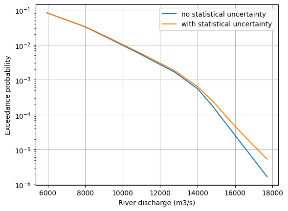
plt.figure()
plt.semilogy(Q_value, Pf_no_stat_uncer, label="no statistical uncertainty")
plt.semilogy(Q_value, Pf_with_stat_uncer, label="with statistical uncertainty")
plt.xlabel("River discharge (m3/s)")
plt.ylabel("Exceedance probability")
plt.grid()
plt.legend()
plt.show()

<matplotlib.legend.Legend at 0x1b22c9679b0>