Visualization of reliability results

In this example, we demonstrate how to visualize the results of a reliability method. The form method is used to estimate the probability of levee failure due to the piping mechanism. This failure mechanism is characterized using the model of Bligh.

Define model

First, let’s we import the necessary classes:

from probabilistic_library import ReliabilityProject, DistributionType, ReliabilityMethod
import matplotlib.pyplot as plt

And the following limit state function:

from utils.models import bligh

To perform a reliability analysis, we create a reliability project and define the limit state function (model):

project = ReliabilityProject()
project.model = bligh

project.model.print()

Model bligh:
Input parameters:
  m
  L
  c_creep
  delta_H
Output parameters:
  Z

We assume the following distributions for the parameters \(m\), \(L\), \(c_{creep}\) and \(\Delta H\):

project.variables["m"].distribution = DistributionType.log_normal
project.variables["m"].mean = 1.76
project.variables['m'].deviation = 0.1

project.variables["L"].distribution = DistributionType.normal
project.variables["L"].mean = 50
project.variables["L"].deviation = 2.5

project.variables["c_creep"].distribution = DistributionType.deterministic
project.variables["c_creep"].mean = 18

project.variables["delta_H"].distribution = DistributionType.gumbel
project.variables["delta_H"].shift = 0.53
project.variables["delta_H"].scale = 0.406

Perform reliability calculations with FORM

The reliability analysis is executed using project.run(), and the results can be accessed via project.design_point. To gain insight into the results, we save the realizations and convergence information.

project.settings.reliability_method = ReliabilityMethod.form
project.settings.relaxation_factor = 0.75
project.settings.maximum_iterations = 50
project.settings.epsilon_beta = 0.01

project.settings.save_realizations = True
project.settings.save_convergence = True

project.run()

project.design_point.print()

Reliability (FORM)
 Reliability index = 3.997
 Probability of failure = 3.214e-05
 Convergence = 0.009351 (converged)
 Model runs = 20
Alpha values:
 m: alpha = 0.1494, x = 1.699
 L: alpha = 0.1347, x = 48.65
 c_creep: alpha = 0, x = 18
 delta_H: alpha = -0.9796, x = 4.591

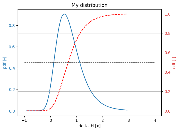
Visualize random variables

Using the plot() method, we can plot the pdf and cdf of a random variable:

project.variables["delta_H"].plot()

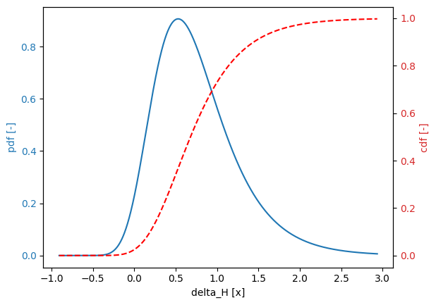
The interval of a random variable used for plotting can be accessed with the get_series() method, which takes into account special points of a random variable, such as the shift in the case of a log-normal distribution.

The method has three optional arguments:

• xmin - user-defined starting point of the interval

• xmax - user-defined end point of the interval

• number_of_points - number of points to be considered

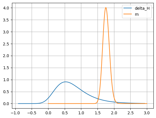
The method can be used to create custom plots:

interval_delta_H = project.variables["delta_H"].get_series()
pdf_delta_H = [project.variables["delta_H"].get_pdf(val) for val in interval_delta_H]

interval_m = project.variables["m"].get_series(xmax=3.0, number_of_points=200)
pdf_m = [project.variables["m"].get_pdf(val) for val in interval_m]

plt.figure()
plt.plot(interval_delta_H, pdf_delta_H, label=project.variables["delta_H"].name)
plt.plot(interval_m, pdf_m, label=project.variables["m"].name)
plt.legend()
plt.grid()
plt.show()

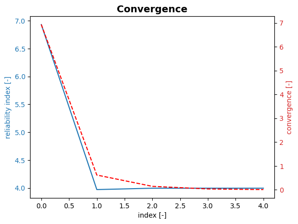
Visualize reliability index and failure probability

Using the plot_convergence() method, we can plot the reliability index (\(\beta\)) and failure probability, corresponding to different model runs:

project.design_point.plot_convergence()

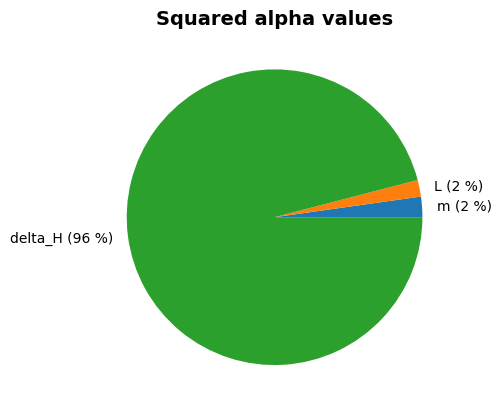
Visualize contribution of random variables

Using the plot_alphas() method, we can visualize the contributions of random variables (\(\alpha^2\)) in a pie chart:

project.design_point.plot_alphas()

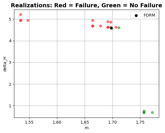
Visualize realizations and design point

Using the plot_realizations() method, we can visualize the realizations and the design point in a two-dimensional space. This is done for the two most contributing variables.

project.design_point.plot_realizations()

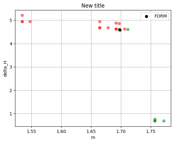
Modify plots

It is possible to modify the plots using the get_plot() method, as demonstrated below:

plt = project.design_point.get_plot_realizations()
plt.title("New title")

Text(0.5, 1.0, 'New title')

plt = project.variables["delta_H"].get_plot()
plt.grid()
plt.plot([-1.0, 4.0], [0.5, 0.5], 'k--', lw=1)
plt.title("My distribution")

Text(0.5, 1.0, 'My distribution')

We can save the figure to a file using savefig():

# plt.savefig("my_distribution.png")