Composite distribution#
A composite distribution, \(F(x)\), is a weighted sum of other distributions:
\(F(x) = \Sigma_{i=1}^{n} w_i \cdot P( X_i \leq x)\) and \(\Sigma_{i=1}^{n} w_i = 1.0\)
where:
\(X_i\) is a random variable
\(w_i\) is a weight associated with random variable \(X_i\)
\(x\) is a realization
In this example, we demonstrate how to define a composite distribution using the probabilistic library.
First, let’s import the necessary packages:
[1]:
from probabilistic_library import DistributionType, ContributingStochast, ConditionalValue, Stochast, StandardNormal
import numpy as np
import matplotlib.pyplot as plt
Defining a composite distribution#
We want to define a composite distribution \(w_{1}\cdot P(X_{1}\leq x) + w_{2} \cdot P(X_{2}\leq x)\), where \(X_1\) is normally distributed with mean \(1.0\) and standard deviation \(0.5\), and \(X_2\) is normally distributed with mean \(4.0\) and standard deviation \(0.3\). The weights are \(0.2\) and \(0.8\), respectively.
To define such a distribution, we first define the variables \(X_1\) and \(X_2\). This is done in the standard way:
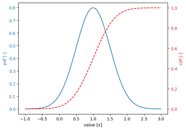
[2]:
x1 = Stochast()
x1.distribution = DistributionType.normal
x1.location = 1.0
x1.scale = 0.5
x1.plot()
[3]:
x2 = Stochast()
x2.distribution = DistributionType.normal
x2.location = 4.0
x2.scale = 0.3
x2.plot()

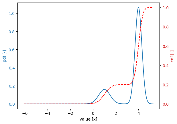
Next, we create a new random variable of composite type and append the two contributing random variables and their corresponding weights using the ContributingStochast class. This results in the composite distribution.
[4]:
w1 = 0.2
w2 = 0.8

stochast = Stochast()
stochast.distribution = DistributionType.composite
stochast.contributing_stochasts.append(ContributingStochast.create(w1, x1))
stochast.contributing_stochasts.append(ContributingStochast.create(w2, x2))

stochast.plot()
Defining a composite conditional distribution#
We can make this example more complex by making the second variable, \(X_2\), conditional on a certain source variable (which is not relevant for this example). This is done as follows:
[5]:
x2 = Stochast()
x2.distribution = DistributionType.normal
x2.conditional = True

source_value = [1.0, 4.0]
mu = [1.0, 4.0]
sigma = [0.5, 0.3]
for ii in range(0, len(source_value)):
    conditional = ConditionalValue()
    conditional.x = source_value[ii]
    conditional.location = mu[ii]
    conditional.scale = sigma[ii]
    x2.conditional_values.append(conditional)
We create the composite random variable:
[6]:
stochast = Stochast()
stochast.distribution = DistributionType.composite
stochast.contributing_stochasts.append(ContributingStochast.create(w1, x1))
stochast.contributing_stochasts.append(ContributingStochast.create(w2, x2))
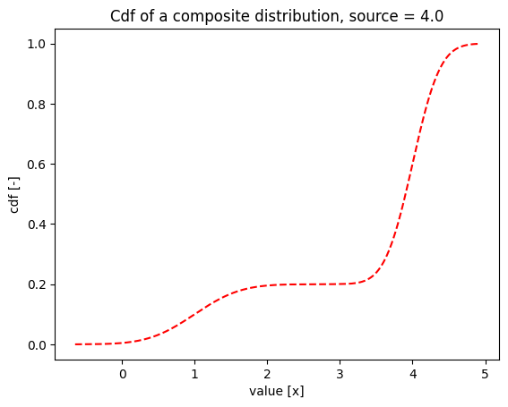
When the source variable is equal to \(4.0\), then the composite distribution is the same as in the first example:
[7]:
source_value = 4.0
p = np.arange(0.0001, 1.0, 0.001)
u = [StandardNormal.get_u_from_p(val) for val in p]
x = [stochast.get_x_from_u_and_source(val, source_value) for val in u]
plt.plot(x, p, 'r--')
plt.xlabel('value [x]')
plt.ylabel('cdf [-]')
plt.title(f'Cdf of a composite distribution, source = {source_value}')
[7]:
Text(0.5, 1.0, 'Cdf of a composite distribution, source = 4.0')
When the source variable is equal to \(1.0\), then the composite distribution is equal to the distribution of \(X_1\):
[8]:
source_value = 1.0
x = [stochast.get_x_from_u_and_source(val, source_value) for val in u]
plt.plot(x, p, 'r--')
plt.xlabel('value [x]')
plt.ylabel('cdf [-]')
plt.title(f'Cdf of a composite distribution, source = {source_value}')
[8]:
Text(0.5, 1.0, 'Cdf of a composite distribution, source = 1.0')
