FORM and correlations#
Reliability calculations with FORM#
In this example, we will demonstrate how to perform reliability calculations using the First Order Reliability Method (FORM).
Define model#
First, let’s import the necessary classes:
[1]:
from probabilistic_library import ReliabilityProject, DistributionType, ReliabilityMethod, StartMethod
Next, we define a simple limit state function:
\(Z = 1.9 - (a+b)\)
This is a linear model involving two variables, \(a\) and \(b\).
[2]:
from utils.models import linear_a_b
To perform a reliability analysis, we create a reliability project and specify the limit state function (model):
[3]:
project = ReliabilityProject()
project.model = linear_a_b

project.model.print()
Model linear_a_b:
Input parameters:
  a
  b
Output parameters:
  Z
We assume that variables \(a\) and \(b\) are uniformly distributed over the interval \([-1, 1]\). This is defined as follows:
[4]:
project.variables["a"].distribution = DistributionType.uniform
project.variables["a"].minimum = -1
project.variables["a"].maximum = 1

project.variables["b"].distribution = DistributionType.uniform
project.variables["b"].minimum = -1
project.variables["b"].maximum = 1
Define reliability method#
We use the reliability method form. We choose the calculation settings: relaxation_factor, maximum_iterations and epsilon_beta.
[ ]:
project.settings.reliability_method = ReliabilityMethod.form
project.settings.relaxation_factor = 0.15
project.settings.maximum_iterations = 50
project.settings.epsilon_beta = 0.01
We can also define the start method, with the following options available: ray_search, one, fixed_value, sensitivity_search, and sphere_search. If the fixed_value option is selected, a start value must be specified for each variable.
[6]:
# fixed_value
project.settings.start_method = StartMethod.fixed_value
project.settings.stochast_settings["a"].start_value = 1.2
project.settings.stochast_settings["b"].start_value = 2.4

# in this example we choose the ray_search method
project.settings.start_method = StartMethod.ray_search
Perform calculations#
We use project.run() to execute the reliability analysis:
[7]:
project.run()
The results are written to project.design_point and consist of:
reliability index \(\beta\)
failure probability \(P_f\)
influence coefficients \(\alpha\)-values
design point \(x\)-values
information about the convergence of FORM
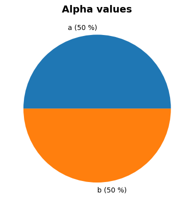
[8]:
project.design_point.print()
project.design_point.plot_alphas()
Reliability (FORM)
 Reliability index = 2.773
 Probability of failure = 0.0028
 Convergence = 0.0088 (converged)
 Model runs = 54
Alpha values:
 a: alpha = -0.7071, x = 0.9501
 b: alpha = -0.7071, x = 0.9501

Contributing design points:
  Reliability (Start point)
   Reliability index = 3.6937
   Probability of failure = 1.104871e-04
   Model runs = 11
  Alpha values:
   a: alpha = -0.4472, x = 0.9014
   b: alpha = -0.8944, x = 0.999
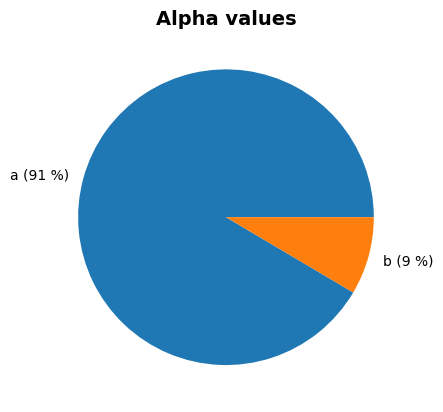
Correlated variables#
In the above example, variables \(a\) and \(b\) are independent. However, it is also possible to introduce a correlation between \(a\) and \(b\). The example below demonstrates this with a partial correlation coefficient of \(0.8\).
[9]:
project.correlation_matrix["a", "b"] = 0.8
project.run()

project.design_point.print()
project.design_point.plot_alphas()
Reliability (FORM)
 Reliability index = 2.0646
 Probability of failure = 0.0195
 Convergence = 0.0084 (converged)
 Model runs = 39
Alpha values:
 a: alpha = -0.9565, x = 0.9517
 b: alpha = -0.2916, x = 0.9478

Contributing design points:
  Reliability (Start point)
   Reliability index = 3.6937
   Probability of failure = 1.104871e-04
   Model runs = 11
  Alpha values:
   a: alpha = -0.4472, x = 0.9014
   b: alpha = -0.8944, x = 0.999