Processing Elevation Data Along Ugrid1d Networks

In this example, we’ll fetch line data describing ditches in the south of the Netherlands and demonstrate several xugrid techniques for working with 1D networks:

• Converting geometries to Ugrid1d networks

• Intersecting edges with external line features

• Refining networks by inserting vertices

• Topology-aware interpolation (nearest neighbor and Laplace)

• Converting node data to edge data

• Network visualization

The dataset contains three components:

• Hydro-objects: center lines representing the ditches.

• Profile points: elevation measurements sampled perpendicular to each center line, describing the cross-sectional profile.

• Profile lines: perpendicular transects connecting the measured points.

We’ll do some basic processing on these data. Our goal is to get an estimate of the bed elevation along the center lines of the ditches.

import matplotlib.patches as patches
import matplotlib.pyplot as plt
import numpy as np
import shapely

import xugrid as xu

The example data consists of three separate GeoDataFrames:

objects, points, profiles = xu.data.hydamo_network()

We will take a look at the center lines and the transects. To get a better idea of the data, we will also zoom in on a 100 by 100 meter window:

xy = (140_270.0, 393_140.0)
dx = dy = 100.0

fig, (ax0, ax1) = plt.subplots(ncols=2, figsize=(10, 5))
objects.plot(ax=ax0, column="type", legend=True)
profiles.plot(ax=ax0, color="red")
ax0.add_patch(patches.Rectangle(xy, dx, dy, fill=False))

objects.plot(ax=ax1, column="type")
profiles.plot(ax=ax1, color="red")
points.plot(ax=ax1, color="black")
ax1.set_xlim(xy[0], xy[0] + dx)
ax1.set_ylim(xy[1], xy[1] + dy)

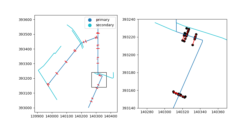
(393140.0, 393240.0)

For spatial analysis, we require sufficient spatial detail – e.g. to compare with a raster digital elevation map (DEM) or for it to serve as model input. We may use shapely to limit the maximum length of linear elements to 25 m. Next, we will generate a Ugrid1d network from the resulting GeoDataFrame.

discretized = shapely.segmentize(objects.geometry, 25.0)
network = xu.Ugrid1d.from_shapely(discretized)

Let’s see whether the conversion to a network topology went well, and what the result of segmentizing is.

fig, ax = plt.subplots()
network.plot(ax=ax)
ax.scatter(*network.node_coordinates.T)

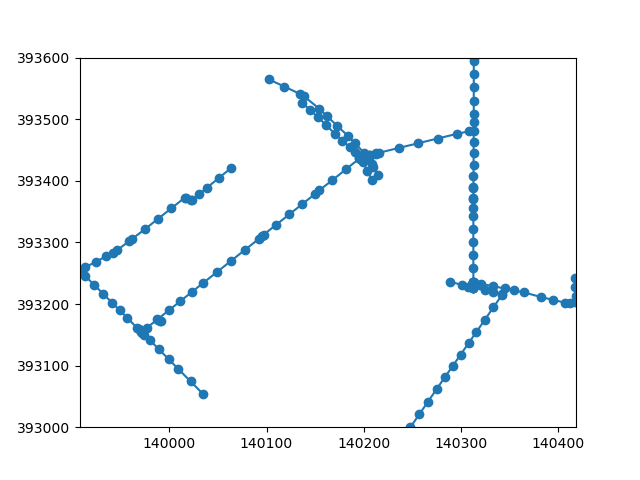
<matplotlib.collections.PathCollection object at 0x7fed68fb2990>

We can see a fairly consistent distribution of nodes. In the next steps, we would like to associate elevation data with nodes of the network. We take the following steps:

• Organize the points per transects and determine its lowest elevation.

• Intersect the center lines with the transects.

• Insert the locations of these intersections as nodes into our network.

• Associate the elevations with the inserted nodes.

Finding the lowest elevation can be done with a pandas groupby. We then add this data to the profile transects, then plot it to check it.

profiles = profiles.set_index("line_id")
profiles["elevation"] = points.groupby("line_id")["elevation"].mean()
profiles.plot(column="elevation", legend=True)

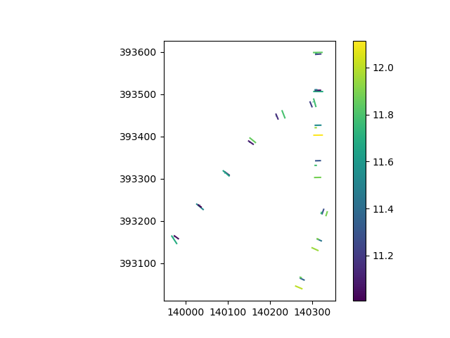
<Axes: >

Not much pattern: a mean elevation centered around 11.5 m above mean sea level and some local variation. Looks like we’ve empirically verified that this part of the Netherlands is indeed rather flat!

For the next step, we will intersect the network with the perpendicular transect lines, and insert the intersections as nodes. The xugrid.intersect_edges() method accepts linework as a numpy array of coordinates.

edges = shapely.get_coordinates(profiles.geometry).reshape((-1, 2, 2))
edge_index, core_index, intersections = network.intersect_edges(edges)

Let’s verify the intersection locations.

fig, ax = plt.subplots()
network.plot(ax=ax, zorder=1)
profiles.plot(ax=ax, zorder=1)
ax.scatter(*network.node_coordinates.T)
ax.scatter(*intersections.T)
ax.set_xlim(xy[0], xy[0] + dx)
ax.set_ylim(xy[1], xy[1] + dy)

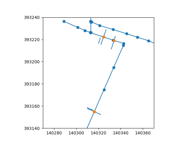
(393140.0, 393240.0)

This looks reasonable. We will now insert the intersections in the network, create a UgridDataArray with the known elevations at the intersections.

refined, insert_index = network.refine_by_vertices(
    intersections, return_index=True, tolerance=1e-6
)
data = np.full(refined.n_node, np.nan)
data[insert_index] = profiles["elevation"].to_numpy()[edge_index]
uda = xu.UgridDataArray.from_data(data, refined, facet="node")

fig, ax = plt.subplots()
refined.plot(ax=ax, zorder=1)
uda.ugrid.plot(ax=ax)

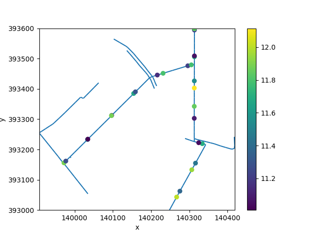
<matplotlib.collections.PathCollection object at 0x7fed5dd98320>

Our end goal is to have elevation data for all edges of the the network. To do so, we can interpolate along the edges, replacing the NoData (NaN) values. Xugrid supports xugrid.UgridDataArrayAccessor.interpolate_na() and xugrid.UgridDataArrayAccessor.laplace_interpolate() for these goals.

Unlike general spatial interpolation methods, these interpolation methods take the topology into account. For example, the nearest distance here is defined along the edges; if there is no connection between two nodes, they does not count towards each other’s nearest neighbors.

Laplace interpolation here smoothly fills gaps by making each unknown value the average of its connected neighbors along the network, similar to how water levels would equilibrate if flowing through the ditches (with a linear hydraulic resistance).

As a final step, we will associate the elevations with the edges, by assigning for each edge the average of its nodes.

nearest = uda.ugrid.interpolate_na()
smooth = uda.ugrid.laplace_interpolate()

edge_nearest = nearest.ugrid.to_edge().mean("nmax")
edge_smooth = smooth.ugrid.to_edge().mean("nmax")

Let’s plot both, and compare the differences.

fig, axes = plt.subplots(ncols=3, figsize=(18, 5))
edge_nearest.ugrid.plot(ax=axes[0], linewidth=3)
edge_smooth.ugrid.plot(ax=axes[1], linewidth=3)
(edge_smooth - edge_nearest).ugrid.plot(ax=axes[2], linewidth=3)
for ax in axes:
    ax.set_aspect(1.0)
axes[0].set_title("Nearest neighbor interpolation")
axes[1].set_title("Laplace interpolation")
axes[2].set_title("Difference")

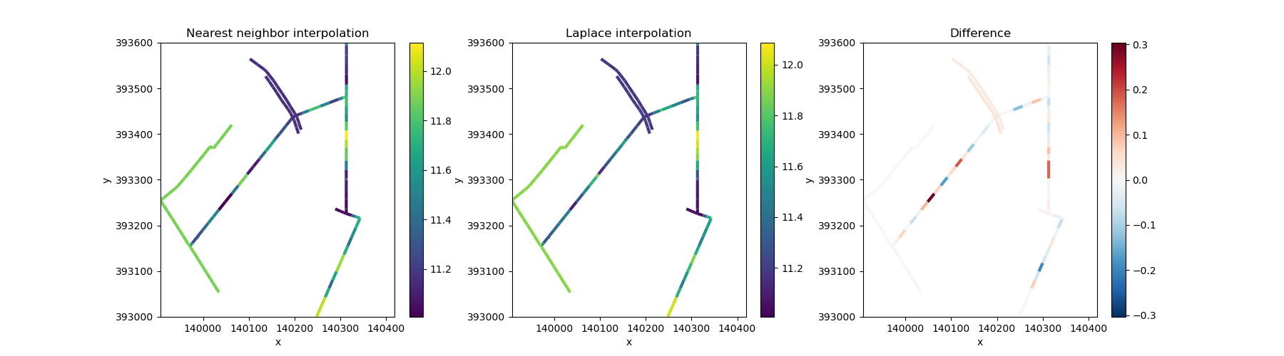
Text(0.5, 1.0, 'Difference')

The actual data here do little to illustrate the interpolation methods! Let’s generate some synthetic data with a clearer pattern. We will assume that the land (and bed) elevation slopes downward in a north-easterly direction with a gradient of 5%.

refine_intersections = refined.node_coordinates[insert_index]
xmax, ymax = refine_intersections.max(axis=0)
synthetic_elevation = (
    xmax - refine_intersections[:, 0] + ymax - refine_intersections[:, 1]
) * 0.05

data = np.full(refined.n_node, np.nan)
data[insert_index] = synthetic_elevation
uda = xu.UgridDataArray.from_data(data, refined, facet="node")

fig, ax = plt.subplots()
refined.plot(ax=ax, zorder=1, linewidth=0.5)
uda.ugrid.plot(ax=ax)

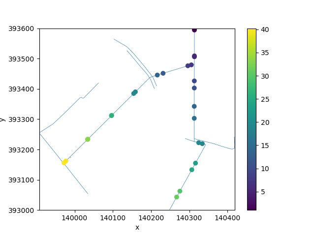
<matplotlib.collections.PathCollection object at 0x7fed5f541520>

Now let’s compare the two interpolation methods. Nearest neighbor interpolation assigns each gap the value of its closest known neighbor along the network. Laplace interpolation creates a smoother solution where each unknown value becomes the average of its connected neighbors— similar to how water levels would equilibrate if flowing through the ditches.

nearest = uda.ugrid.interpolate_na()
smooth = uda.ugrid.laplace_interpolate()

edge_nearest = nearest.ugrid.to_edge().mean("nmax")
edge_smooth = smooth.ugrid.to_edge().mean("nmax")

fig, axes = plt.subplots(ncols=3, figsize=(18, 5))
edge_nearest.ugrid.plot(ax=axes[0], linewidth=3)
edge_smooth.ugrid.plot(ax=axes[1], linewidth=3)
(edge_smooth - edge_nearest).ugrid.plot(ax=axes[2], linewidth=3)

for ax in axes:
    ax.set_aspect(1.0)

axes[0].set_title("Nearest neighbor interpolation")
axes[1].set_title("Laplace interpolation")
axes[2].set_title("Difference")

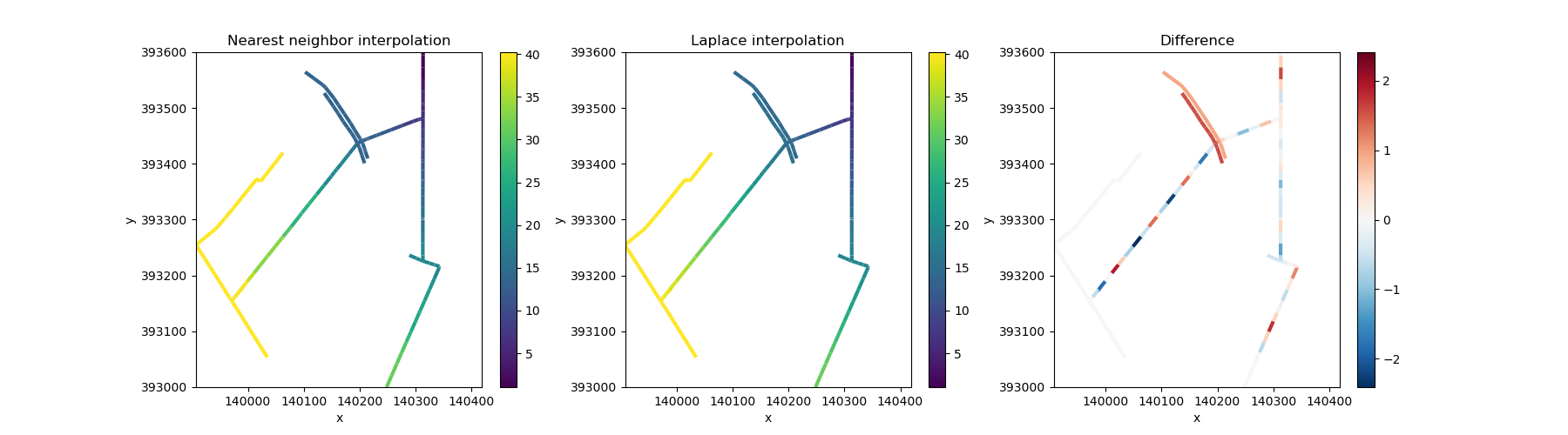
Text(0.5, 1.0, 'Difference')

We can now clearly see how reaches without data are filled “along” the network topology. The difference plot shows that Laplace interpolation produces smoother transitions, while nearest neighbor creates more abrupt changes where the nearest known value switches from one transect to another.