Note
Go to the end to download the full example code.
Regridding#
Introduction#
Most MODFLOW 6 packages have spatial data arrays as input. These arrays are discrete: they are defined over the simulation grid and contain values associated to each cell.
Regridding these package means: create a new package with spatial data arrays defined over a different grid. Computing what the values in these new arrays should be, is done by xugrid.
xugrid will compute a regridded array based on:
the original array
the original discretization (this is described in the coordinates of the original arry)
the new discretization
a regridding method
More information on the available regridding methods can be found in the xugrid documentation https://deltares.github.io/xugrid/user_guide.html
The regridding method that should be used depends on the property being regridded. For example a point-based property (whose value do not depend intrinsically on the grid block size) such as temperature or density can be regridded by an averaging approach (for upscaling) or sampling (for downscaling). Volume-based properties (whose values do depend on the grid block size) include (water) mass and pore volume of a gridblock, and the regridding method should be chosen to reflect that. Finally regridding methods for conductivity-like properties follow the rules for parallel or serial resistors- at least when the tensor rotation angles are constant or comparable in the involved gridblocks.
Note that the different regridding methods may have a different output domain when regridding: if the original array has no-data values in some cells, then the output array may have no-data values as well, and where these end up depends on the chosen regridding method. Also note that regridding is only possible in the xy-plane, and not across the layer dimension. The output array will have the same number of layers as the input array.
Obtaining the final (i)domain#
In many real-world models, some cells will be inactive or marked as “vertical
passthrough” (VPT) in the idomain array of the simulation. Some packages
require that all cells that are inactictive or VPT in idomain are excluded
from the package as well. An example is the imod.mf6.NodePropertyFlow
package: cells that are inactive or VPT in idomain, should not have
conductivity data in the npf package. Therefore at the end of the regridding
process, a final step consists in enforcing consistency between those of
idomain and all the packages. This is a 2-step process:
for cells that do not have inputs in crucial packages like npf or storage, idomain will be set to inactive.
for cells that are marked as inactive or VPT in idomain, all package inputs will be removed from all the packages
This synchronization step between idomain and the packages is automated, and it is carried out when calling regrid_like on the simulation object or the model object. There are 2 caveats:
the synchronization between idomain and the package domains is done on the model-level. If we have a simulation containing both a flow model and a transport model then idomain for flow is determined independent from that for transport. These models may therefore end up using different domains (this may lead to undesired results, so a manual synchronization may be necessary between the flow regridding and the transport regridding) This manual synchronization can be done using the “mask_all_packages” function- this function removes input from all packages that are marked as inactive or VPT in the idomain passed to this method.
The idomain/packages synchronization step is carried out when regridding a model, and when regridding a model it will use default methods for all the packages. So if you have regridded some packages yourself with non-default methods, then these are not taken into account during this synchonization step.
Regridding using default methods#
The regrid_like function is available on packages, models and simulations. When the default methods are acceptable, regridding the whole simulation is the most convenient from a user-perspective.
import imod

tmpdir = imod.util.temporary_directory()

original_simulation = imod.data.hondsrug_simulation(tmpdir / "hondsrug_saved")
To reduce computational overhead for this example, we are going to clip off most of the timesteps.
original_simulation = original_simulation.clip_box(time_max="2010-01-01")
Let’s take a look at the original discretization:
original_simulation["GWF"]["dis"]
We want to regrid this to the following target grid:
import xarray as xr

import imod

dx = 100
dy = -100
xmin = 237500.0
xmax = 250000.0
ymin = 559000.0
ymax = 564000.0
target_grid = imod.util.empty_2d(
    dx=dx, dy=dy, xmin=xmin, xmax=xmax, ymin=ymin, ymax=ymax
)

target_grid
This is a grid of nans, and we require a grid of ones, which can create with xarray:
target_grid = xr.ones_like(target_grid)

target_grid
Now regrid the simulation (without recharge):
regridded_simulation = original_simulation.regrid_like("regridded", target_grid)
Let’s look at the discretization again:
regridded_simulation["GWF"]["dis"]
All packages have been regridded, for example the NPF package:
regridded_simulation["GWF"]["npf"]
Let’s make a comparison plot of the hydraulic conductivities:
import matplotlib.pyplot as plt
import numpy as np

fig, axes = plt.subplots(nrows=2, sharex=True)
plot_kwargs = {"colors": "viridis", "levels": np.linspace(0.0, 100.0, 21), "fig": fig}

imod.visualize.spatial.plot_map(
    original_simulation["GWF"]["npf"]["k"].sel(layer=3), ax=axes[0], **plot_kwargs
)
imod.visualize.spatial.plot_map(
    regridded_simulation["GWF"]["npf"]["k"].sel(layer=3), ax=axes[1], **plot_kwargs
)

axes[0].set_ylabel("original")
axes[1].set_ylabel("regridded")
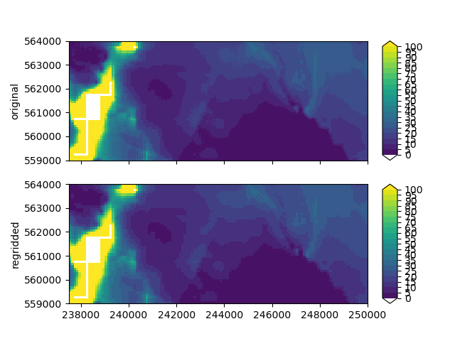
Text(28.472222222222243, 0.5, 'regridded')
Regridding using non-default methods#
When non-default methods are used for one or more packages, these should be regridded separately. In that case, the most convenient approach is likely:
pop the packages that should use non-default methods from the source simulation (the popping is optional, and is only recommended for packages whose presence is not mandatory for validation.)
regrid the source simulation: this takes care of all the packages that should use default methods.
regrid the package(s) where you want to use non-standard rergridding methods indivudually starting from the packages in the source simulation
insert the custom-regridded packages to the regridded simulation (or replace the package regridded with default methods with the one you just regridded with non-default methods if it was not popped)
In code, consider an example where we want to regrid the recharge package using non default methods then we would do the following. First we’ll load some example simulation. There is a separate example contained in Regional model that you should look at if you are interested in the model building
Set up the input needed for custom regridding. Create a regridder weight-cache. This object can (and should) be reused for all the packages that undergo custom regridding at this stage.
from imod.util.regrid import RegridderWeightsCache

regrid_cache = RegridderWeightsCache()

regrid_cache
<imod.util.regrid.RegridderWeightsCache object at 0x0000019B2A1BD580>
Next, we’ll remove the recharge package and obtain it as a variable. We’ll do this for later use.
original_rch_package = original_simulation["GWF"].pop("rch")

original_rch_package
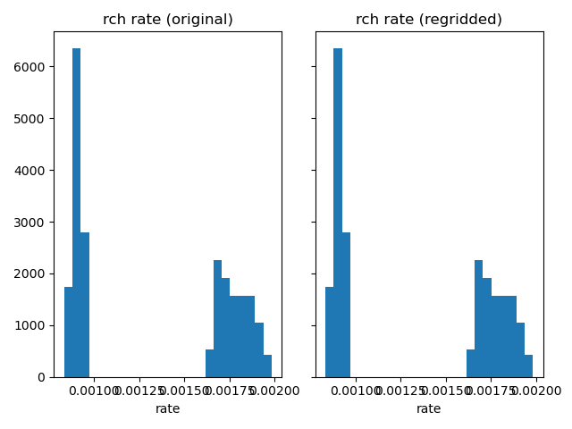
Regrid the recharge package with a custom regridder. In this case we opt for the centroid locator regridder. This regridder is similar to using a “nearest neighbour” lookup.
from imod.common.utilities.regrid import RegridderType
from imod.mf6.regrid import RechargeRegridMethod

regridder_types = RechargeRegridMethod(rate=(RegridderType.CENTROIDLOCATOR,))

regridded_recharge = original_rch_package.regrid_like(
    target_grid,
    regrid_cache=regrid_cache,
    regridder_types=regridder_types,
)

regridded_recharge
Next, add the recharge package to the regridded simulation
regridded_simulation["GWF"]["rch"] = regridded_recharge

# We can also reattach the original again
original_simulation["GWF"]["rch"] = original_rch_package
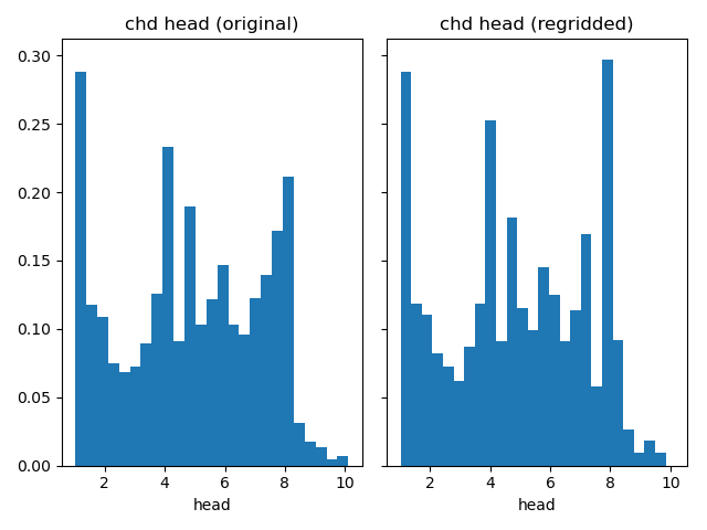
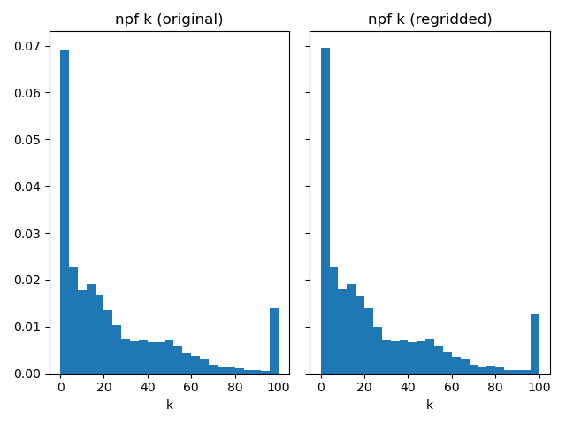
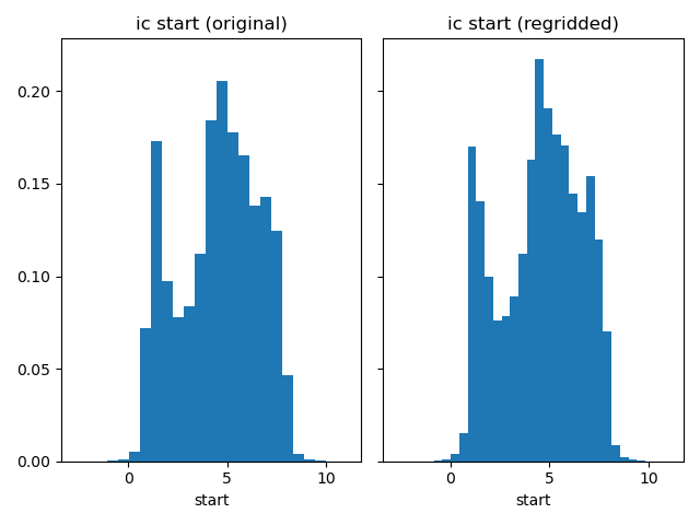
Comparison with histograms#
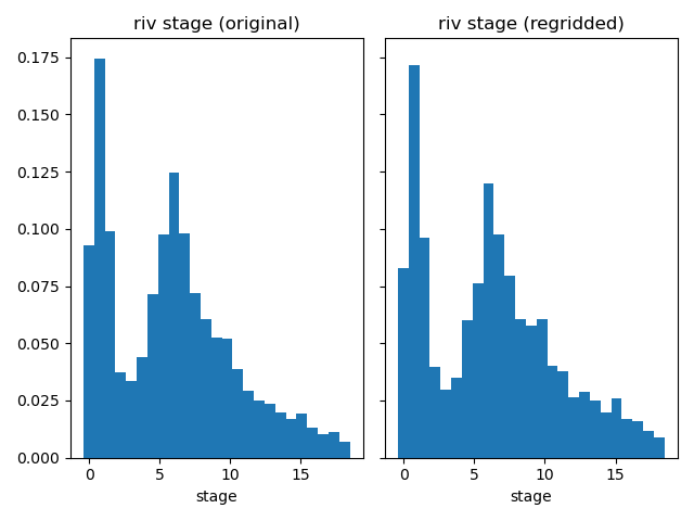
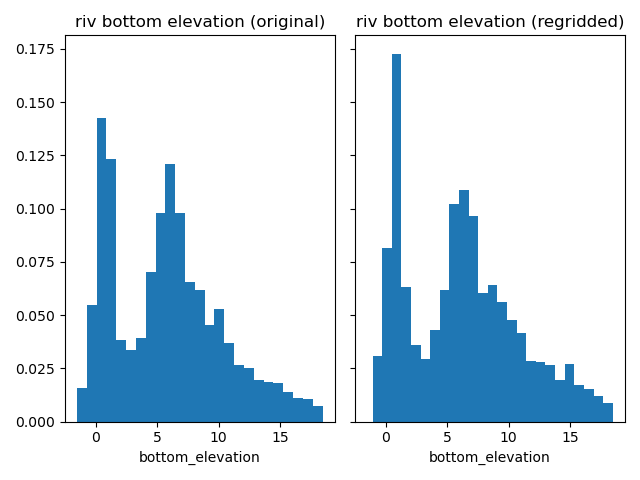
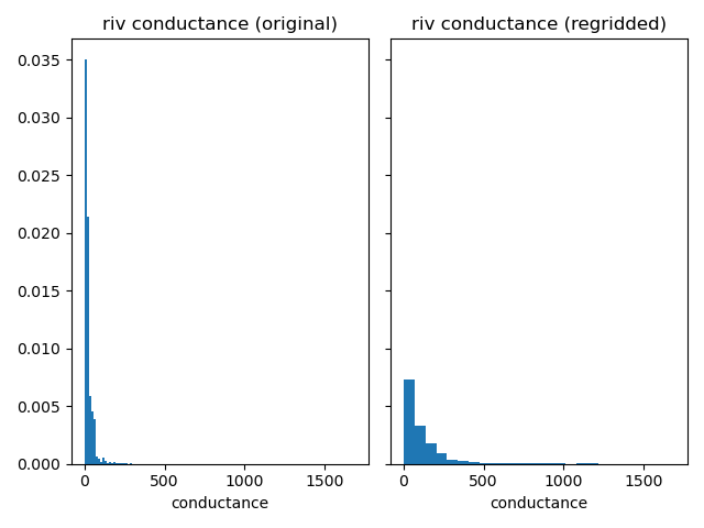
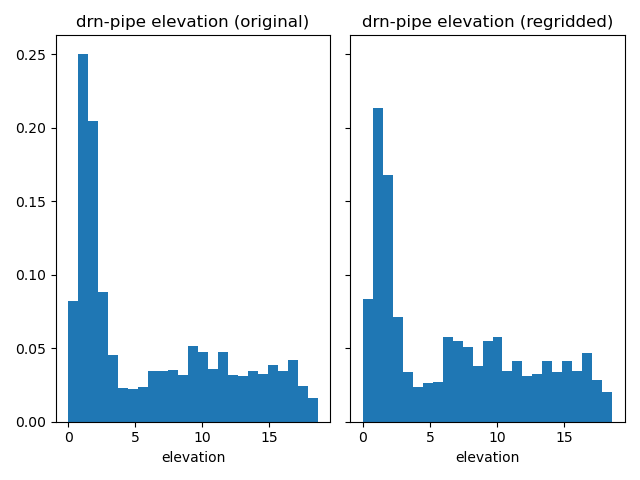
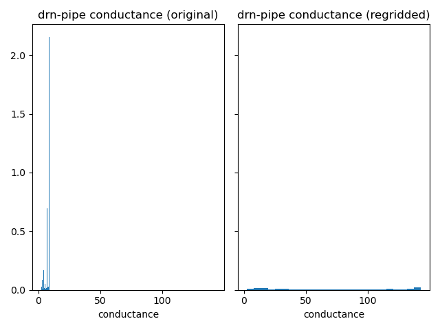
In the next segment we will compare the input of the models on different
grids. We advice to always check how your input is regridded. In this example
we upscaled grid, many input parameters are regridded with a mean method.
This means that their input range is reduced, which can be seen in tailings in
the histograms becoming shorter
def plot_histograms_side_by_side(array_original, array_regridded, title):
    """This function creates a plot of normalized histograms of the 2 input
    DataArray. It plots a title above each histogram."""
    _, (ax0, ax1) = plt.subplots(1, 2, sharex=True, sharey=True, tight_layout=True)
    array_original.plot.hist(ax=ax0, bins=25, density=True)
    array_regridded.plot.hist(ax=ax1, bins=25, density=True)
    ax0.title.set_text(f"{title} (original)")
    ax1.title.set_text(f"{title} (regridded)")
Compare constant head arrays.
plot_histograms_side_by_side(
    original_simulation["GWF"]["chd"]["head"],
    regridded_simulation["GWF"]["chd"]["head"],
    "chd head",
)
Compare horizontal hydraulic conductivities.
plot_histograms_side_by_side(
    original_simulation["GWF"]["npf"]["k"],
    regridded_simulation["GWF"]["npf"]["k"],
    "npf k",
)
Compare vertical hydraulic conductivities.
plot_histograms_side_by_side(
    original_simulation["GWF"]["npf"]["k33"],
    regridded_simulation["GWF"]["npf"]["k33"],
    "npf k33",
)

Compare starting heads.
plot_histograms_side_by_side(
    original_simulation["GWF"]["ic"]["start"],
    regridded_simulation["GWF"]["ic"]["start"],
    "ic start",
)
Compare river stages.
plot_histograms_side_by_side(
    original_simulation["GWF"]["riv"]["stage"],
    regridded_simulation["GWF"]["riv"]["stage"],
    "riv stage",
)
Compare river bottom elevations.
plot_histograms_side_by_side(
    original_simulation["GWF"]["riv"]["bottom_elevation"],
    regridded_simulation["GWF"]["riv"]["bottom_elevation"],
    "riv bottom elevation",
)
Compare riverbed conductance.
plot_histograms_side_by_side(
    original_simulation["GWF"]["riv"]["conductance"],
    regridded_simulation["GWF"]["riv"]["conductance"],
    "riv conductance",
)
Compare recharge rates.
plot_histograms_side_by_side(
    original_simulation["GWF"]["rch"]["rate"],
    regridded_simulation["GWF"]["rch"]["rate"],
    "rch rate",
)
Compare drainage elevations.
plot_histograms_side_by_side(
    original_simulation["GWF"]["drn-pipe"]["elevation"],
    regridded_simulation["GWF"]["drn-pipe"]["elevation"],
    "drn-pipe elevation",
)
Compare drain conductances.
plot_histograms_side_by_side(
    original_simulation["GWF"]["drn-pipe"]["conductance"],
    regridded_simulation["GWF"]["drn-pipe"]["conductance"],
    "drn-pipe conductance",
)
Compare simulation outputs#
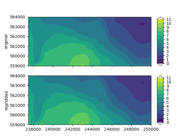
Let’s compare outputs now.
# Write simulation
original_simulation.write(tmpdir / "original")
# Run and open heads
original_simulation.run()
hds_original = original_simulation.open_head()

hds_original
regridded_simulation.write(tmpdir / "regridded", validate=False)
regridded_simulation.run()
hds_regridded = regridded_simulation.open_head()

hds_regridded
Let’s make a comparison plot of the regridded heads.
fig, axes = plt.subplots(nrows=2, sharex=True)
plot_kwargs = {"colors": "viridis", "levels": np.linspace(0.0, 11.0, 12), "fig": fig}

imod.visualize.spatial.plot_map(
    hds_original.isel(layer=6, time=-1), ax=axes[0], **plot_kwargs
)
imod.visualize.spatial.plot_map(
    hds_regridded.isel(layer=6, time=-1), ax=axes[1], **plot_kwargs
)

axes[0].set_ylabel("original")
axes[1].set_ylabel("regridded")
Text(28.472222222222243, 0.5, 'regridded')
A note on regridding conductivity#
In the npf package, it is possible to use for definining the conductivity tensor:
1 array (K)
2 arrays (K and K22)
3 arrays (K, K22, K33)
If 1 array is given the tensor is called isotropic. Defining only K gives the same behavior as specifying K, K22 and K33 with the same value. When regridding, K33 has a default method different from that of K and K22, but it can only be applied if K33 exists in the source model in the first place. So it is recommended to introduce K33 as a separate array in the source model even if it is isotropic. Also note that default regridding methods were chosen assuming that K and K22 are roughly horizontal and K33 roughly vertical. But this may not be the case if the input arrays angle2 and/or angle3 have large values.
Regridding boundary conditions#
Special care must be taken when regridding boundary conditions, and it is recommended that users verify the balance output of a regridded simulation and compare it to the original model. If the regridded simulation is a good representation of the original simulation, the mass contributions on the balance by the different boundary conditions should be comparable in both simulations. To achieve this, it may be necessary to tweak the input or the regridding methods. An example of this is upscaling recharge (so the target grid has coarser cells than the source grid). Its default method is averaging, with the following rules:
if a cell in the source grid is inactive in the source recharge package (meaning no recharge), it will not count when averaging. So if a target cell has partial overlap with one source recharge cell, and the rest of the target cell has no overlap with any source active recharge cell, it will get the recharge of the one cell it has overlap with. But since the target cell is larger, this effectively means the regridded recharge will be more in the regridded simulation than it was in the source simulation
but we do the same regridding this time assigning a zero recharge to cells without recharge then the averaging will take the zero-recharge cells into account and the regridded recharge will be the same as the source recharge.
A note on regridding transport#
Transport simulations can be unstable if constraints related to the grid Peclet number and the courant number are exceeded. This can easily happen when regridding. It may be necessary to reduce the simulation’s time step size especially when downscaling, to prevent numerical issues. Increasing dispersivities or the molecular diffusion constant can also help to stabilize the simulation. Inversely, when upscaling, a larger time step size can be acceptable.
Unsupported packages#
Some packages cannot be regridded. This includes the Lake package and the UZF package. Such packages should be removed from the simulation before regridding, and then new packages should be created by the user and then added to the regridded simulation.
Listing all default regridding methods#
MODFLOW 6#
This code snippet prints all default methods:
import inspect
import sys
from dataclasses import asdict

import pandas as pd


def collect_regrid_methods(classes: list):
    """Collect all regrid methods from all list of package classes."""
    regrid_method_setup = {
        "package name": [],
        "array name": [],
        "method name": [],
        "function name": [],
    }
    regrid_method_table = pd.DataFrame(regrid_method_setup)
    counter = 0
    for obj in classes:
        if hasattr(obj, "_regrid_method"):
            package_name = obj.__name__
            regrid_methods = asdict(obj.get_regrid_methods())
            for array_name in regrid_methods.keys():
                method_name = regrid_methods[array_name][0].name
                function_name = ""
                if len(regrid_methods[array_name]) > 0:
                    function_name = regrid_methods[array_name][1]
                regrid_method_table.loc[counter] = (
                    package_name,
                    array_name,
                    method_name,
                    function_name,
                )
                counter = counter + 1

    # Set multi index to group with packages
    regrid_method_table = regrid_method_table.set_index(["package name", "array name"])
    return regrid_method_table


# Get all classes in the imod.mf6 module (e.g.
# :class:`imod.mf6.NodePropertyFlow`, :class:`imod.mf6.GroundwaterFlowModel`,
# :class:`imod.mf6.River`)
mf6_classes = [
    obj for _, obj in inspect.getmembers(sys.modules["imod.mf6"], inspect.isclass)
]

mf6_regrid_methods = collect_regrid_methods(mf6_classes)

# Pandas by default displays at max 60 rows, which this table exceeds.
nrows = mf6_regrid_methods.shape[0]
# Configure pandas to increase the max amount of displayable rows.
pd.set_option("display.max_rows", nrows + 1)
# Display rows:
mf6_regrid_methods
MetaSWAP#
Let’s list all default regridding methods for all MetaSWAP packages:
msw_classes = [
    obj for _, obj in inspect.getmembers(sys.modules["imod.msw"], inspect.isclass)
]

msw_regrid_methods = collect_regrid_methods(msw_classes)

msw_regrid_methods
Total running time of the script: (1 minutes 25.413 seconds)