Note
Go to the end to download the full example code.
Unstructured Grids#
MODFLOW 6 supports unstructured grids. Unlike raster data, the connectivity of unstructured grids is irregular. This means that the number of neighboring cells is not constant; for structured grids, every cell has 4 neighbors (in 2D), or 6 neighbors (in 3D).
The package we use to handle unstructured grids is called xugrid. It is a Python package that provides a data structure for unstructured grids, and allows for plotting and analysis of these grids. It is built on top of xarray <https://xarray.pydata.org/en/stable/>`_, so handling data is similar to how you would handle raster data in xarray, with some differences.
Let’s first load some sample data from xugrid.data module. The example data is a triangular grid of the elevation of the Netherlands.
import xugrid as xu

elevation = xu.data.elevation_nl()

elevation
Note that this data is stored differently than a raster dataset. We don’t see
an x- and a y-dimension here. So where is this spatial information?
It’s in this grid attribute, which is accesses via the ugrid accessor.
This is a special accessor that provides access to the unstructured grid
properties of the dataset.
grid = elevation.ugrid.grid
grid
<xarray.Dataset> Size: 255kB
Dimensions:            (mesh2d_nFaces: 5248, nmax_face: 3, mesh2d_nNodes: 2790)
Coordinates:
    mesh2d_node_x      (mesh2d_nNodes) float64 22kB ...
    mesh2d_node_y      (mesh2d_nNodes) float64 22kB ...
    mesh2d_face_x      (mesh2d_nFaces) float64 42kB ...
    mesh2d_face_y      (mesh2d_nFaces) float64 42kB ...
Dimensions without coordinates: mesh2d_nFaces, nmax_face, mesh2d_nNodes
Data variables:
    mesh2d             int32 4B ...
    mesh2d_face_nodes  (mesh2d_nFaces, nmax_face) float64 126kB 138.0 ... 1.9...
Attributes:
    Conventions:  CF-1.8 UGRID-1.0
The grid has a number of properties, such as the number of cells, the coordinates of the vertices, and the connectivity of the cells. The latter is very important when dealing with unstructured grids, as it defines how the cells are connected to each other. This is different from structured grids, where you don’t need to specify this as there connectivity follows from the rows and columns. Let’s take a look at the connectivity of this unstructured grid:
grid.format_connectivity_as_dense(grid.face_face_connectivity)
array([[  89,   -1,   -1],
       [ 244,  362,  367],
       [  15,  279,  335],
       ...,
       [2041, 3617, 5246],
       [ 528, 3618, 5245],
       [ 528, 3617, 3640]], shape=(5248, 3))
This shows the connectivity of the cells in the grid. Each row represents a cell, and the columns represent the neighboring cells. Because this is a grid with triangles, we can see three columns in the connectivity matrix. -1 indicates that a cell is not connected to a neighbour. For example, the first cell is only connected to one cell.
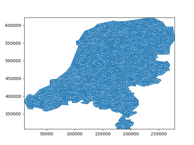
You can imagine that plotting unstructured grids is quite a hassle, as you need to provide quite some information to the plotting function. Fortunately, the xugrid package provides a convenient way to plot unstructured grids. Let’s plot the grid:
grid.plot()
<matplotlib.collections.LineCollection object at 0x0000019B29FA83B0>
We can plot the grid with the data values as well:
elevation.ugrid.plot()
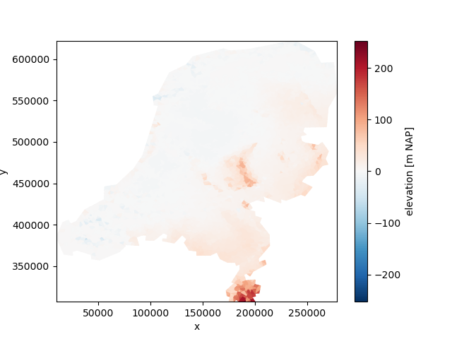
<matplotlib.collections.PolyCollection object at 0x0000019B29FAD3D0>
Note that we need to call the ugrid accessor to plot the data. This is
because the data is stored in a different format than raster data, and we need
to tell python that xugrid needs to be used for plotting, and not the regular
xarray plotting methods.
We can make calculations just like we would do with raster data. For example, we can calculate the mean elevation of the Netherlands:
mean_elevation = elevation.mean()
mean_elevation
Or if we want to compute a grid of the elevation 100 meters below the surface:
elevation_100m_below = elevation - 100
elevation_100m_below.ugrid.plot()
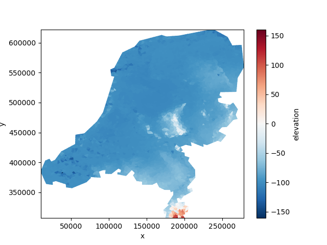
<matplotlib.collections.PolyCollection object at 0x0000019B2646B7D0>
We can use this data to be the bottom elevation of a MODFLOW 6 layered unstructured discretization (DISV). For that we need to assign a layer coordinate as iMOD Python requires a layer dimension to be present on the bottom and idomain variables.
bottom = elevation_100m_below.expand_dims("layer").assign_coords(layer=[1])
Finally we need to create an idomain variable that indicates which cells are active. For this example we will assume all cells are active, so we can just create an idomain variable with all ones. We can do this with the xu.ones_like function.
idomain = xu.ones_like(bottom).astype(int)
Now we can create a MODFLOW 6 unstructured discretization (DISV) object using
the imod.mf6.VerticesDiscretization class. We will create a
discretization with one model layer.
from imod.mf6 import VerticesDiscretization

disv = VerticesDiscretization(top=elevation, bottom=bottom, idomain=idomain)
Note: we just created a model discretization on a triangular grid. This means that a line connecting two cell centers is rarely perfectly orthogonal to the cell edge. This causes mass balance errors. A voronoi grid would be a better choice for a model discretization, as it ensures that the cell centers are perfectly orthogonal to the cell edges. Luckily for us, xugrid has functionality to tesselate a grid into voronoi cells.
voronoi_grid = grid.tesselate_centroidal_voronoi()
voronoi_grid.plot()
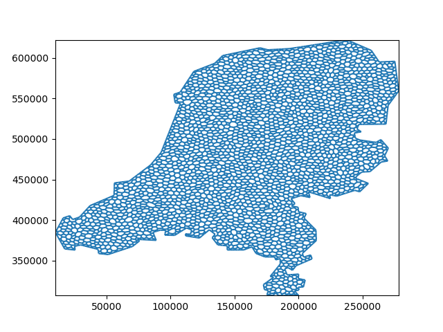
<matplotlib.collections.LineCollection object at 0x0000019B1C51BCE0>
We can use this voronoi grid to create a new MODFLOW 6 unstructured discretization (DISV) object. iMOD Python has regridding functionality to regrid the top, bottom and idomain variables to the new grid.
For that, iMOD Python regridding functionality requires a UgridDataArray instead of a Ugrid2d, so we create a UgridDataArray with the voronoi grid.
from imod.util import RegridderWeightsCache, ones_like_ugrid

voronoi_uda = ones_like_ugrid(voronoi_grid)

disv_voronoi = disv.regrid_like(voronoi_uda, RegridderWeightsCache())
disv_voronoi
Other packages like the imod.mf6.Drainage package, accept both structured and
unstructured grids.
The drain elevation requires a layer dimension. We can use the idomain to broadcast the data to include the layer dimension.
drain_elevation = disv_voronoi["idomain"] * disv_voronoi["top"]
drain_elevation
We also need to create a conductance variable for the
imod.mf6.Drainage package. The conductance variable is a measure of
how much water can flow through a cell. The areas of the cells are used to
calculate the conductance, and can be be obtained from its grid.
resistance = 1  # Example resistance value in days
conductance = disv_voronoi["idomain"] * voronoi_grid.area / resistance
We can now use these variables to create a imod.mf6.Drainage package object.
from imod.mf6 import Drainage

drainage = Drainage(
    elevation=drain_elevation,
    conductance=conductance,
)
drainage
That wraps up the example of how to use unstructured grids in iMOD Python. For more information on how to manipulate unstructured grids and how to make selections, please refer to the xugrid documentation.
Total running time of the script: (0 minutes 3.234 seconds)