Note
Go to the end to download the full example code.
Raster data and xarray#
Geospatial data primarily comes in two forms: raster data and vector data. This guide focuses on the first.
Raster data consists of rows and columns of rectangular cells. Their location in space is defined by the number of rows, the number of columns, a cell size along the rows, a cell size along the columns, the origin (x, y), and optionally rotation (x, y) – an affine matrix.
Typical examples of file formats containing raster data are:
GeoTIFF
ESRII ASCII
netCDF
IDF
In groundwater modeling, data commonly stored in raster format are:
Layer topology: the tops and bottoms of geohydrological layers
Layer properties: conductivity of aquifers and aquitards
Model output: heads or cell by cell flows
These data consist of values for every single cell. Xarray provides many conveniences for such data, such as plotting or selecting. To demonstrate, we’ll get some sample data provided with the imod package.
import xarray as xr
import imod

elevation = imod.data.ahn()["ahn"]
elevation
Two dimensions: x, y#
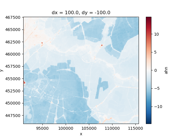
This dataset represents some surface elevation in the west of the Netherlands, in the form of an xarray DataArray.
Xarray provides a “rich” representation of this data, note the x and y coordinates are shown above. We can use these coordinates for plotting, selecting, etc.
elevation.plot()
<matplotlib.collections.QuadMesh object at 0x0000019B16A5E5A0>
This creates an informative plot.
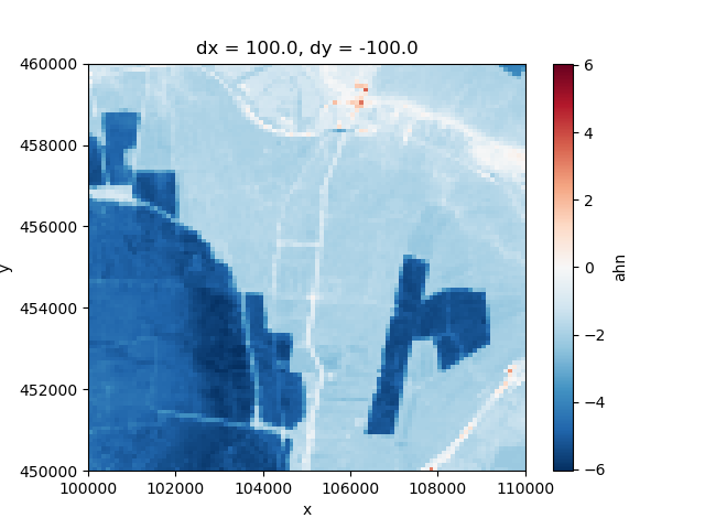
We can also easily make a selection of a 10 by 10 km square, and plot the result:
selection = elevation.sel(x=slice(100_000.0, 110_000.0), y=slice(460_000.0, 450_000.0))
selection.plot()
<matplotlib.collections.QuadMesh object at 0x0000019B2655B500>
More dimensions#
Raster data can also be “stacked” to represent additional dimensions, such as height or time. Xarray is fully N-dimensional, and can directly represent these data.
Let’s start with a three dimensional example: a geohydrological layer model.
layermodel = imod.data.hondsrug_layermodel()
layermodel
This dataset contains multiple variables. We can take a closer look at the the “top” variable, which represents the top of every layer.
top = layermodel["top"]
top
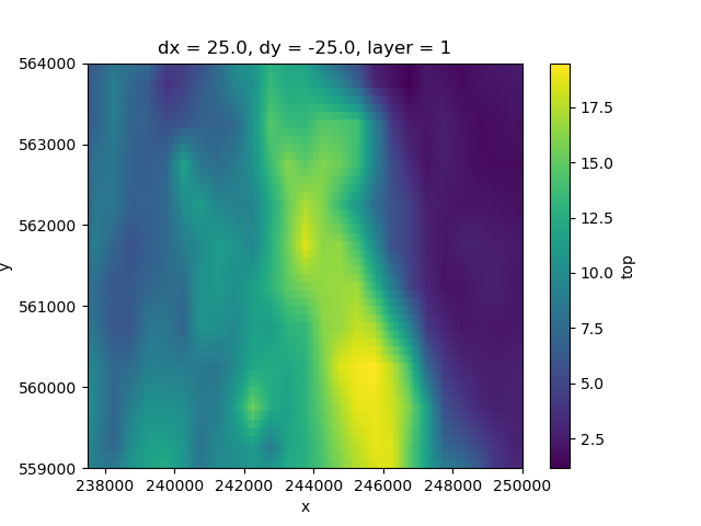
This DataArray has three dimensions: layer, y, x. We can’t make a planview plot of this entire dataset: every (x, y) locations has as many values as layers. A single layer can be selected and shown as follows:
top.sel(layer=1).plot()
<matplotlib.collections.QuadMesh object at 0x0000019B2655A6C0>
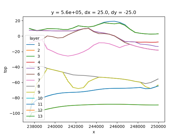
Xarray doesn’t favor specific dimensions. We can select a value along the y-axis just as easily, to create a cross-section.
section = top.sel(y=560_000.0, method="nearest")
section.plot.line(x="x")
[<matplotlib.lines.Line2D object at 0x0000019B2652EF90>, <matplotlib.lines.Line2D object at 0x0000019B2655B1A0>, <matplotlib.lines.Line2D object at 0x0000019B29F97B30>, <matplotlib.lines.Line2D object at 0x0000019B29F96F00>, <matplotlib.lines.Line2D object at 0x0000019B29F96EA0>, <matplotlib.lines.Line2D object at 0x0000019B29F96CF0>, <matplotlib.lines.Line2D object at 0x0000019B29F96C60>, <matplotlib.lines.Line2D object at 0x0000019B29F96B40>, <matplotlib.lines.Line2D object at 0x0000019B29F96990>, <matplotlib.lines.Line2D object at 0x0000019B29F96930>, <matplotlib.lines.Line2D object at 0x0000019B29F965D0>, <matplotlib.lines.Line2D object at 0x0000019B29F96480>, <matplotlib.lines.Line2D object at 0x0000019B29FCF4A0>]
Xarray provides us a lot of convenience compared to working with traditional two dimensional rasters: rather than continuously loop over the data of single timesteps or layers, we can process them in a single command.
For example, to compute the thickness of every layer:
thickness = layermodel["top"] - layermodel["bottom"]
thickness
This is easily multiplied, then summed over the layer dimensions to provide us a map of the total transmissivity:
transmissivity = layermodel["k"] * thickness
total = transmissivity.sum("layer")
total.plot()
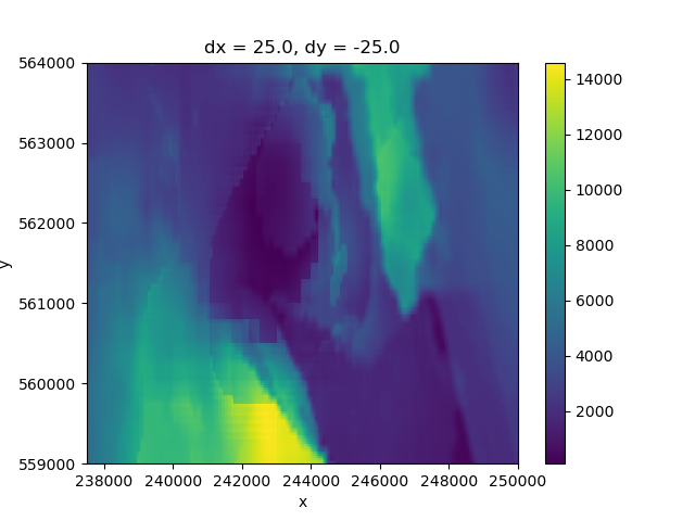
<matplotlib.collections.QuadMesh object at 0x0000019B1DEBD070>
Input and output#
The imod package started as a collection of functions to read IDF files
into xarray DataArrays. By convention, IDF files store the coordinates
of the extra dimensions (layer, time) in the file name.
imod.idf.save() will automatically generate these names from
a DataArray.
Let’s demonstrate by writing the transmissivity computed above to IDF. (We’ll do this in a temporary directory to keep things tidy.)
tempdir = imod.util.temporary_directory()
imod.idf.save(tempdir / "transmissivity", transmissivity)
Note
tempdir is a Python pathlib.Path object. These objects
are very convenient for working with paths; we can easily check
if paths exists, join paths with /, etc.
Let’s check which files have been written in the temporary directory:
filenames = [path.name for path in tempdir.iterdir()]
print("\n".join(filenames))
transmissivity_l1.idf
transmissivity_l10.idf
transmissivity_l11.idf
transmissivity_l12.idf
transmissivity_l13.idf
transmissivity_l2.idf
transmissivity_l3.idf
transmissivity_l4.idf
transmissivity_l5.idf
transmissivity_l6.idf
transmissivity_l7.idf
transmissivity_l8.idf
transmissivity_l9.idf
Just as easily, we can read all IDFs back into a single DataArray. We can do so by using a wildcard. These wildcards function according to the rules of Glob via the python glob module.
Note that every IDF has to have identical x-y coordinates: files with different cell sizes or extents will not be combined automatically.
back = imod.idf.open(tempdir / "*.idf")
back
These glob patterns are quite versatile, and may be used to filter as well.
selection = imod.idf.open(tempdir / "transmissivity_l[1-5].idf")
selection
Rather commonly, the paths of the IDFs are not named according to consistent
rules. In such cases, we can manually specify how the name should be
interpreted via the pattern argument.
back = imod.idf.open(tempdir / "*.idf", pattern="{name}_l{layer}")
back
See the documenation of imod.idf.open() for more details.
Other raster formats#
IDF is one raster format, but there are many more.
imod.rasterio.open() wraps the rasterio Python package (which in
turn wraps GDAL) to provide access to many GIS raster formats.
imod.rasterio.open() and imod.rasterio.save() work exactly
the same as the respective IDF functions, except they write to a different
format.
For example, to write the transsmisivity to GeoTIFF:
imod.rasterio.save(tempdir / "transmissivity.tif", transmissivity)
filenames = [path.name for path in tempdir.iterdir()]
print("\n".join(filenames))
transmissivity_l1.idf
transmissivity_l1.tif
transmissivity_l10.idf
transmissivity_l10.tif
transmissivity_l11.idf
transmissivity_l11.tif
transmissivity_l12.idf
transmissivity_l12.tif
transmissivity_l13.idf
transmissivity_l13.tif
transmissivity_l2.idf
transmissivity_l2.tif
transmissivity_l3.idf
transmissivity_l3.tif
transmissivity_l4.idf
transmissivity_l4.tif
transmissivity_l5.idf
transmissivity_l5.tif
transmissivity_l6.idf
transmissivity_l6.tif
transmissivity_l7.idf
transmissivity_l7.tif
transmissivity_l8.idf
transmissivity_l8.tif
transmissivity_l9.idf
transmissivity_l9.tif
Note imod.rasterio.save() will split the extension off the path,
infer the GDAL driver, attach the additional coordinates to the file name,
and re-attach the extension.
netCDF#
The final format to discuss here is netCDF. Two dimensional raster files are convenient for viewing, as every file corresponds with a single “map view” in a GIS viewer. However, they are not convenient for storing many timesteps or many layers: especially long running simulations will generate hundreds, thousands, or even millions of files.
netCDF is a file format specifically designed for multi-dimensional data, and allows us to conveniently bundle all data in a single file. Xarray objects can directly be written to netCDF, as the data model of xarray itself is based on the netCDF data model.
With netCDF, there is no need to encode the different dimension labels in the the name: they are stored directly in the file instead.
layermodel.to_netcdf(tempdir / "layermodel.nc")
back = xr.open_dataset(tempdir / "layermodel.nc")
back
Coordinate reference systems (CRS)#
Reprojection from one CRS to another is a common frustration. Since the data in an xarray DataArray is always accompanied by its x and y coordinates, we can easily reproject the data. See the example Reproject data.
MODFLOW 6#
iMOD Python’s MODFLOW 6 module supports raster data in the form of xarray
DataArrays. It will interpret data with an "x" and "y" coordinate
automatically as data on structured grid. Let’s create a structured
discretization package (DIS) first. Note that MODFLOW 6 requires top to
have only one layer, so we select the first layer of the layer model.
Furthermore, the idomain is required to be an integer array, so we convert it
to an integer type.
import imod

top = layermodel["top"].sel(layer=1)
idomain = layermodel["idomain"].astype(int)

dis = imod.mf6.StructuredDiscretization(
    top=top, bottom=layermodel["bottom"], idomain=idomain
)
dis
Great! We can now use this discretization in a MODFLOW 6 model. Say we want to
create a drainage package for overland flow. We can use the top array as drain
elevation, but we only want drain cells in the first layer, where idomain ==
1.
layer = layermodel.coords["layer"]
is_top_layer_and_active = (layer == 1) & (idomain == 1)
drain_elevation = layermodel["top"].where(is_top_layer_and_active)
Next, we need to create a conductance array. The conductance is a measure of how much water can flow through a cell. We can use the areas of the cells to compute a conductance array.
area = layermodel["dx"] * layermodel["dy"] * -1
resistance = 1  # Example resistance value in days
conductance_value = area / resistance
conductance = conductance_value.where(is_top_layer_and_active)
We can now create a drainage package object:
drn = imod.mf6.Drainage(
    elevation=drain_elevation,
    conductance=conductance,
)
drn
Total running time of the script: (0 minutes 4.200 seconds)