Note
Go to the end to download the full example code.
Time series data and Pandas#
Handling time series is major part of geohydrology and groundwater modeling. Time series data come in more than one form:
Time series linked to a point location, for example a measured groundwater level at a specific location.
Time series of a spatially continuous nature, for example model output of calculated head for a specific model layer.
We typically represent time series data at points as a
pandas.DataFrame, despite the (apparent) match with GeoDataFrames.
The issue is that a GeoDataFrame has to store the geometry for every row: this
means many duplicated geometries. Fortunately, pandas’ group by
(split-apply-combine) functionality provides a (fairly) convenient way of
working with time series data of many points.
Pandas provides many tools for working with time series data, such as:
Input and output to many tabular formats, such as CSV or Excel;
Data selection;
Filling or interpolating missing data;
Resampling to specific frequencies;
Plotting.
Timeseries at point locations#
iMOD represents time series at points in an IPF format. This format stores its data as:
A “mother” file containing the x and y coordinates of the point. Each point can be associated with a timeseries with a label.
A timeries file for every point.
These files can be read via imod.formats.ipf.read(). The read function
will read the mother file, and follow its labels, reading every associated
timeseries file as well. Finally, these are merged into a single large table;
the properties of the point (e.g. the x,y coordinates) are duplicated for every
row.
Note
This may seem wasteful, but:
There are few data structures available for storing point data with associated time series. For example: xarray can store the point location as coordinates, but every point will need to share its time axis – the same time window for every point and the same time resolution.
There are equally few file formats suitable for this data. A single large table is supported by many file formats.
Pandas group by functionality is quite fast.
Example: Head observations#
Let’s load some example data. We’ll load some head observations. This is a
large dataset, originally stored in the IPF format. This dataset has a similar
form to what imod.formats.ipf.read() would return.
import imod

heads = imod.data.head_observations()
heads
We can see that the data is stored in a long format, with duplicate entries for each time. Let’s do some selections to showcase some functionality of pandas. Let’s first compute filter depth, which is the difference between the surface_elevation and the top of the filter. Note: “Meetpunt tov m NAP” = surface elevation, “filt_top” = top of the filter.
filter_depth = heads["Meetpunt tov m NAP"] - heads["filt_top"]
filter_depth
0        0.57
1        0.57
2        0.57
3        0.57
4        0.57
         ...
60374    7.44
60375    7.44
60376    7.44
60377    7.44
60378    7.44
Length: 60379, dtype: float64
The original dataset is very large, so let’s limit ourselves to only head observations close to surface elevation. Let’s say the first 20 cm below surface.
heads_shallow = heads.loc[filter_depth < 0.2]
heads_shallow = heads_shallow.sort_values(by="time")
Let’s plot the head observations for these shallow observations over time with a separate line for each filter.
import matplotlib.pyplot as plt

fig, ax = plt.subplots()
for key, group in heads_shallow.groupby("id"):
    ax = group.plot(x="time", y="head", ax=ax, label=key)
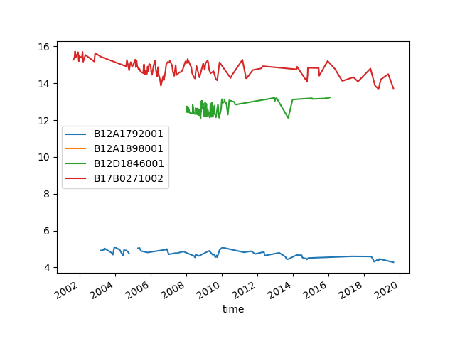
It seems one line disappeared. Let’s count the number of observations per filter. We can see that one of the filters has only one observation, making it hard to draw a line.
heads_shallow.groupby("id")["head"].count()
id
B12A1792001     72
B12A1898001      1
B12D1846001    113
B17B0271002    124
Name: head, dtype: int64
Let’s check whether these head observations were all measured at the same date. We can groupby time and count the number of observations per time.
n_obs_per_time = heads_shallow.groupby("time")["id"].count()
n_obs_per_time
time
2001-07-16    1
2001-08-14    1
2001-09-14    1
2001-09-28    1
2001-10-14    1
             ..
2018-11-14    1
2018-12-13    1
2019-05-14    1
2019-08-28    1
2019-08-30    1
Name: id, Length: 297, dtype: int64
We can see in the printed summary that most dates have only one observation, and that the last two dates are only two days apart. This is likely caused by observations on inconsistent dates.
Let’s see if there are some dates with more than one observation.
n_obs_per_time.unique()
array([1, 2])
We can see that there are some dates with two observations. Lets’s see which dates those are:
n_obs_per_time.loc[n_obs_per_time == 2]
time
2004-08-14    2
2004-10-14    2
2005-04-14    2
2005-04-28    2
2005-05-14    2
2005-10-28    2
2007-10-14    2
2008-12-14    2
2009-01-14    2
2009-01-28    2
2009-08-28    2
2009-09-14    2
2009-09-28    2
2014-09-29    2
2014-10-14    2
Name: id, dtype: int64
MODFLOW 6#
iMOD Python’s imod.mf6.Well and imod.mf6.LayeredWell classes
require their data to be provided as points. However, these require the rates
to be provided on consistent timesteps amongst all points. This means that the
data has to be resampled to a consistent frequency. This is done for the user
when calling imod.mf6.Well.from_imod5_data() or
imod.mf6.LayeredWell.from_imod5_data().
Total running time of the script: (0 minutes 1.518 seconds)