Quick start#

These are the examples in the index page of the iMOD Python user guide. The examples are used to demonstrate the features of iMOD Python and how to use them. This file is meant to test if the index page is working correctly and to provide a quick overview of the examples available in the user guide.

Let’s first create some raster data to work with.

import xarray as xr
import xugrid as xu

import imod

elevation_uda = xu.data.elevation_nl()
# Drop unnecessary coords. These coords are also stored in elevation_uda.ugrid.grid
elevation_uda = elevation_uda.drop_vars(["mesh2d_face_x", "mesh2d_face_y"])

part = elevation_uda.ugrid.sel(
    x=slice(100_000.0, 200_000.0), y=slice(400_000.0, 500_000.0)
)

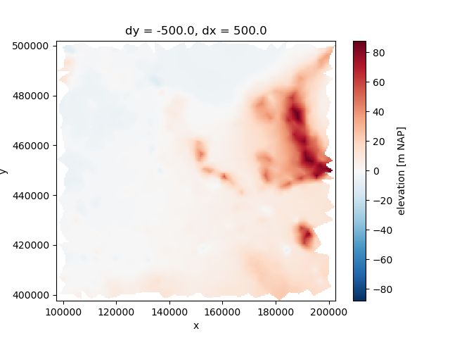
Make structured grid

resolution = 500.0
xmin, ymin, xmax, ymax = part.ugrid.grid.bounds
structured_grid = imod.util.empty_2d(resolution, xmin, xmax, resolution, ymin, ymax)

# Interpolate
regridder = xu.BarycentricInterpolator(part, structured_grid)
interpolated_elevation = regridder.regrid(part)

# Plot
interpolated_elevation.plot.imshow()

<matplotlib.image.AxesImage object at 0x0000016F389124B0>

Save to GeoTIFF

# Create a temporary directory to store the data
tmp_dir = imod.util.path.temporary_directory()
tmp_dir.mkdir(parents=True, exist_ok=True)
interpolated_elevation.rio.to_raster(tmp_dir / "elevation.tif")

Seamlessly integrate your GIS rasters or meshes with MODFLOW 6, by using xarray and xugrid arrays, for structured and unstructured grids respectively, to create grid-based model packages.

# Open Geotiff with elevation data as xarray DataArray
elevation = imod.rasterio.open(tmp_dir / "elevation.tif")
elevation.load()

# Create idomain grid
layer_template = xr.DataArray([1, 1, 1], dims=("layer",), coords={"layer": [1, 2, 3]})
idomain = layer_template * xr.ones_like(elevation).astype(int)
# Deactivate cells with NoData
idomain = idomain.where(elevation.notnull(), 0)

# Compute bottom elevations of model layers
layer_thickness = xr.DataArray(
    [10.0, 20.0, 10.0], dims=("layer",), coords={"layer": [1, 2, 3]}
)
bottom = elevation - layer_thickness.cumsum(dim="layer")

# Create MODFLOW 6 DIS package
dis_pkg = imod.mf6.StructuredDiscretization(
    idomain=idomain, top=elevation, bottom=bottom.transpose("layer", "y", "x")
)

Assign wells based on x, y coordinates and filter screen depths, instead of layer, row and column:

import pandas as pd

# Specify well locations
x = [150_200.0, 160_800.0]
y = [450_300.0, 460_200.0]

# Specify well screen depths
screen_top = [0.0, 0.0]
screen_bottom = [-4.0, -10.0]

# Specify flow rate, which changes over time.
weltimes = pd.date_range("2000-01-01", "2000-01-03", freq="2D")
well_rates_period1 = [0.5, 1.0]
well_rates_period2 = [2.5, 3.0]
rate = xr.DataArray(
    [well_rates_period1, well_rates_period2],
    coords={"time": weltimes},
    dims=("time", "index"),
)

# Now construct the Well package
wel_pkg = imod.mf6.Well(
    x=x, y=y, rate=rate, screen_top=screen_top, screen_bottom=screen_bottom
)

# iMOD Python will take care of the rest and assign the wells to the correct model
# layers upon writing the model. It will furthermore distribute well rates based
# on transmissivities. To verify how wells will be assigned to model layers before
# writing the entire simulation, you can use the following command:
wel_mf6_pkg = wel_pkg.to_mf6_pkg(idomain, elevation, bottom, k=1.0)

# Wells have been distributed across two model layers based on screen depths.
print(wel_mf6_pkg["cellid"])

# Well rates have been distributed based on screen overlap
print(wel_mf6_pkg["rate"])

<xarray.DataArray 'cellid' (ncellid: 4, dim_cellid: 3)> Size: 96B
array([[  1, 104, 106],
       [  1,  84, 127],
       [  2, 104, 106],
       [  2,  84, 127]])
Coordinates:
  * ncellid     (ncellid) int64 32B 0 1 2 3
  * dim_cellid  (dim_cellid) <U6 72B 'layer' 'row' 'column'
    x           (ncellid) float64 32B 1.502e+05 1.608e+05 1.502e+05 1.608e+05
    y           (ncellid) float64 32B 4.503e+05 4.602e+05 4.503e+05 4.602e+05
<xarray.DataArray 'rate' (ncellid: 4, time: 2)> Size: 64B
array([[0.28073287, 1.40366435],
       [0.58867207, 1.7660162 ],
       [0.21926713, 1.09633565],
       [0.41132793, 1.2339838 ]])
Coordinates:
  * ncellid  (ncellid) int64 32B 0 1 2 3
    x        (ncellid) float64 32B 1.502e+05 1.608e+05 1.502e+05 1.608e+05
    y        (ncellid) float64 32B 4.503e+05 4.602e+05 4.503e+05 4.602e+05
  * time     (time) datetime64[ns] 16B 2000-01-01 2000-01-03

MODFLOW 6 requires that all stress periods are defined in the time discretization package. However, usually boundary conditions are defined at insconsistent times. iMOD Python can help you to create a time discretization package that is consistent, based on all the unique times assigned to the boundary conditions.

simulation = imod.mf6.Modflow6Simulation("example")
simulation["gwf"] = imod.mf6.GroundwaterFlowModel()
simulation["gwf"]["dis"] = dis_pkg
simulation["gwf"]["wel"] = wel_pkg

# Create a time discretization based on the times assigned to the packages.
# Specify the end time of the simulation as one of the additional_times
simulation.create_time_discretization(additional_times=["2000-01-07"])

# Note that timesteps in well package are also inserted in the time
# discretization
print(simulation["time_discretization"].dataset)

<xarray.Dataset> Size: 48B
Dimensions:              (time: 2)
Coordinates:
  * time                 (time) datetime64[ns] 16B 2000-01-01 2000-01-03
Data variables:
    timestep_duration    (time) float64 16B 2.0 4.0
    n_timesteps          int64 8B 1
    timestep_multiplier  float64 8B 1.0

Regrid MODFLOW 6 models to different grids, even from structured to unstructured grids. iMOD Python takes care of properly scaling the input parameters. You can also configure scaling methods yourself for each input parameter, for example when you want to upscale drainage elevations with the minimum instead of the average.

new_unstructured_grid = part
sim_regridded = simulation.regrid_like("regridded", new_unstructured_grid)

# Notice that discretization has converted to VerticesDiscretization (DISV)
print(sim_regridded["gwf"]["dis"])

VerticesDiscretization
<xarray.Dataset> Size: 79kB
Dimensions:        (layer: 3, mesh2d_nFaces: 1238)
Coordinates:
  * layer          (layer) int64 24B 1 2 3
  * mesh2d_nFaces  (mesh2d_nFaces) int64 10kB 0 1 2 3 4 ... 1234 1235 1236 1237
Data variables:
    idomain        (layer, mesh2d_nFaces) int64 30kB 1 1 1 1 1 1 ... 1 1 1 1 1 1
    top            (mesh2d_nFaces) float64 10kB 7.708 18.72 ... 12.31 11.52
    bottom         (layer, mesh2d_nFaces) float64 30kB -2.292 8.724 ... -28.48

To reduce the size of your model, you can clip it to a bounding box. This is useful for example when you want to create a smaller model for testing purposes.

sim_clipped = simulation.clip_box(
    x_min=125_000, x_max=175_000, y_min=425_000, y_max=475_000
)

You can even provide states for the model, which will be set on the model boundaries of the clipped model. Create a grid of zeros, which will be used to set as heads at the boundaries of clipped parts.

head_for_boundary = xr.zeros_like(idomain, dtype=float).where(idomain > 0)
states_for_boundary = {"gwf": head_for_boundary}

sim_clipped = simulation.clip_box(
    x_min=125_000,
    x_max=175_000,
    y_min=425_000,
    y_max=475_000,
    states_for_boundary=states_for_boundary,
)

# Notice that a Constant Head (CHD) package has been created for the clipped
# model.
print(sim_clipped["gwf"])

GroundwaterFlowModel(
    listing_file=None,
    print_input=False,
    print_flows=False,
    save_flows=False,
    newton=False,
    under_relaxation=False,
){
    'dis': StructuredDiscretization,
    'wel': Well,
    'chd_clipped': ConstantHead,
}

Total running time of the script: (1 minutes 3.201 seconds)

Gallery generated by Sphinx-Gallery

Quick start#

This Page