Lazy evaluation

A powerful feature of xarray is lazy evaluation. Lazy evaluation means that expressions are delayed until the results are needed. In a nutshell, lazy evaluation has the following advantages for us:

• Lazy evaluation frees us from having to load all data into memory in one go. We can work with larger-than-memory datasets without having to manually divide the datasets into smaller, manageable pieces.

• Lazy evaluation allows us to easily parallellize computations. This can speed up computations considerably depending on the available number of cores.

Lazy evaluation can be contrasted with eager evaluation. In eager evaluation with xarray, all data always exists in RAM memory, and computations are performed immediately. Typical cases of when results are needed is when data has to be visualized or when the data has to be saved to disk.

We will explain these concepts with a number of examples.

import dask.array
import numpy as np
import xarray as xr

import imod

lazy_da = xr.DataArray(dask.array.ones(5), dims=["x"])
lazy_result = lazy_da + 1

When we run the lines above, we evaluate the expression lazy_result = lazy_da + 1. In eager evaluation, this means a value of 1 is added to every element; in delayed evaluation, the expression is stored instead in a graph of tasks. In xarray, delayed evaluation is taken care of by dask, an open source Python library for (parallel) scheduling and computing.

We can identify the DataArray as lazy, since its .data attribute shows a dask array rather than a numpy array.

lazy_result.data

Array Chunk Bytes 40 B 40 B Shape (5,) (5,) Dask graph 1 chunks in 2 graph layers Data type float64 numpy.ndarray

We can take a look at the graph of tasks as follows:

lazy_result.data.visualize()

Note

The show function here is required for the online documentation. If you’re running the examples interactively, the line above will show you a picture of the graph, and defining and calling show() can be ommitted.

def show():
    # Show the latest png generated by dask.visualize with matplotlib. This is
    # required because the sphinx image scraper currently only supports
    # matplotlib and mayavi and will not capture the output of
    # dask.visualize().
    import matplotlib.image as mpimg
    import matplotlib.pyplot as plt

    _, ax = plt.subplots()
    ax.set_axis_off()
    ax.imshow(mpimg.imread("mydask.png"))


show()

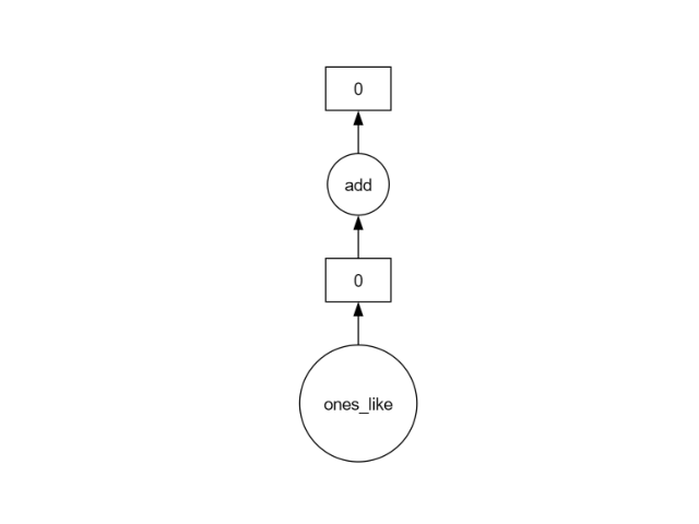
We can see a very simple graph with two tasks:

• create the array of ones;

• add a value of 1 to every element.

Let’s constrast this with eager evaluation. Rather than creating the data as a dask array, we will create it as an ordinary numpy array.

eager_da = xr.DataArray(np.ones(5), dims=["x"])
eager_result = eager_da + 1
eager_result.data

array([2., 2., 2., 2., 2.])

The data is an numpy array. Since the actual values of the elements of the array are in memory, we also get a preview of the element values.

See also the xarray documentation on parallel computing with dask.

Delayed computation and (i)MODFLOW files

The input and output functions in the imod package have been written to work with xarray’s delayed evaluation. This means that opening IDFs or MODFLOW6 will not load the data from the files into memory until they are needed.

Let’s grab some example results, store them in a temporarily directory, and open them:

result_dir = imod.util.temporary_directory()
imod.data.twri_output(result_dir)
head = imod.mf6.open_hds(result_dir / "twri.hds", result_dir / "twri.grb")

All time steps are available, but not loaded. Instead, a graph of tasks has been defined. Let’s take a look at the tasks:

head.data.visualize()
show()

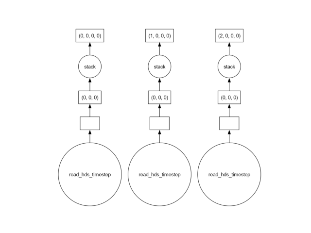
We might want to perform a computation for every time step. Let’s assume we would want to compute the mean head for every time step:

mean_head = head.mean(["y", "x"])

We can take a look at the graph, and see that the dask are fully independent of each other:

mean_head.data.visualize()
show()

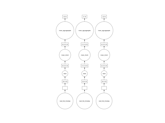
This means the computation is embarrassingly parallel. Every task can be computed independently of the other by the individual CPUs of your computer.

Dask will automatically distribute tasks over your CPUs, and manage the tasks so that memory usage does not exceed maximum RAM. This goes well most of the time, but not always; refer to the Pitfalls section below.

Chunk size and memory layout

Computer memory and data storage are best thought of a one-dimensional arrays of bits (even though the hardware might be actually multi-dimensional behind the scenes).

Pitfalls

There are a number of pitfalls to be aware of when working with dask and lazy evaluation. A primary pitfall is not taking the chunk (and memory) layout into mind. For working with MODFLOW models, this is typically operations that operate over the time dimension. Because of the file formats, MODFLOW data is chunked over the time dimension.

Concretely, this means that the following code can be very slow for large datasets:

points = [(0.0, 0.0), (1.0, 1.0), (2.0, 2.0)]
samples = [head.sel(x=x, y=y, method="nearest") for (x, y) in points]

samples[0].data.visualize()
show()

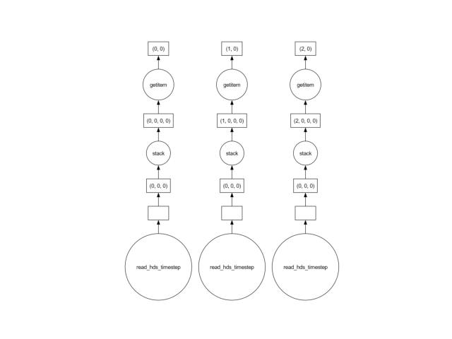
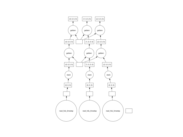
The reason is that in the line above, a single x-y point is extracted at a time. To extract this single point, the entire dataset must be loaded into memory! Generally, the solution is to use a vectorized approach, selecting all the points “at once”.

x = [0.0, 1.0, 2.0]
y = [0.0, 1.0, 2.0]
samples = head.sel(x=x, y=y, method="nearest")

In these lines, the chunk is loaded, all point values for a single time step are extracted and store; then the next chunk is loaded, etc. Because the call is vectorized, dask can optimize the selection, and figure out that it should extract all values and load the chunks only once. We can verify this by taking a look at the task graph again:

samples.data.visualize()
show()

There are cases where the data cannot be loaded in a vectorized manner, or cases where the scheduling goes haywire. In this case, a straightforward solution is to fallback to eager evaluation (with numpy arrays instead of dask arrays). This can be done at any time by simply calling .compute():

eager_head = head.compute()

This has the obvious downside that the entire dataset needs to fit in memory.

However, the following lines are relatively fast again, since the entire dataset has already been loaded into memory this time around:

points = [(0.0, 0.0), (1.0, 1.0), (2.0, 2.0)]
samples = [eager_head.sel(x=x, y=y, method="nearest") for (x, y) in points]

Annoyingly, the VSCode interactive Python interpreter does not cooperate well with every dask scheduler. If you’re working in VSCode, and either performance seems slow or memory usage is very high, try running your script outside of VSCode.