Note
Go to the end to download the full example code.
Topsystem: from 2D map to 3D model#
iMOD Python has multiple features to help you define the topsystem of the groundwater system. With “topsystem” we mean all forcings which act on the top of the groundwater system. These are usually either meteorological (precipitation & evapotranspiration) or hydrological (rivers, ditches, lakes, sea) in nature. In MODFLOW 6 these are usually simulated with the DRN, RIV, GHB, and RCH package. This data is usually provided as planar grids (x, y) without any vertical dimension. This user guide will show you how to allocate these forcings across model layers to grid cells and how to distribute conductances for Robin-like boundary conditions (RIV, DRN, GHB) over model layers. We will demonstrate this with the RIV package, as this package supports all options for allocating cells and distributing conductances. A subset of options are available for the DRN, GHB, and RCH packages.
Example data#
Let’s load the data first. We have a layer model containing a basic hydrogeological schemitization of our model, so the tops and bottoms of model layers, the hydraulic conductivity (k), and which cells are active (idomain=1) or vertical passthrough (idomain=-1).
import imod

layer_model = imod.data.hondsrug_layermodel_topsystem()

layer_model
Furthermore we have planar grid of river, containing a river stage, bed elevation and conductance.
planar_river = imod.data.hondsrug_planar_river()

planar_river
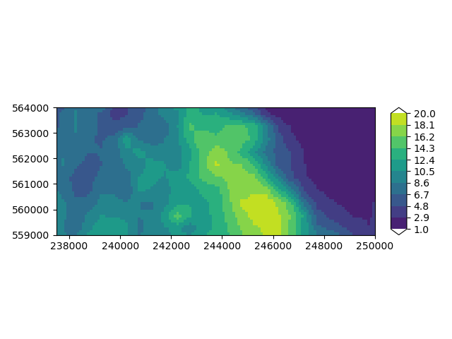
Let’s plot the top elevation of the model on a map. You can see we have a ridge roughly the centre of the model, sided by two low-lying areas.
import numpy as np

imod.visualize.plot_map(
    layer_model["top"].sel(layer=1), "viridis", np.linspace(1, 20, 11)
)
(<Figure size 640x480 with 2 Axes>, <Axes: >)
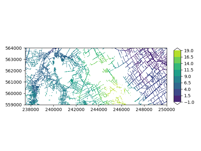
Let’s plot the river stages on a map. You can see most rivers are located in the low-lying areas.
imod.visualize.plot_map(planar_river["stage"], "viridis", np.linspace(-1, 19, 9))
(<Figure size 640x480 with 2 Axes>, <Axes: >)
Allocate river cells#
Let’s allocate river cells across model layers to cells.
from imod.prepare import ALLOCATION_OPTION, allocate_riv_cells

riv_allocated, _ = allocate_riv_cells(
    allocation_option=ALLOCATION_OPTION.at_elevation,
    active=layer_model["idomain"] == 1,
    top=layer_model["top"],
    bottom=layer_model["bottom"],
    stage=planar_river["stage"],
    bottom_elevation=planar_river["bottom"],
)
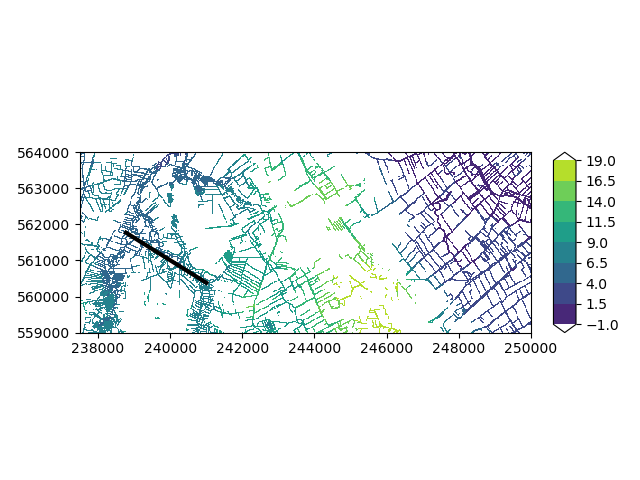
Let’s take a look at what we just produced. Since we are dealing with information with depth, it is simplest to make a crosssection plot. For that, we first have to select a crosssection.
import geopandas as gpd
from shapely.geometry import LineString

geometry = LineString([[238725, 561800], [241050, 560350]])

# Define overlay
overlays = [
    {"gdf": gpd.GeoDataFrame(geometry=[geometry]), "edgecolor": "black", "linewidth": 3}
]
# Plot
imod.visualize.plot_map(
    planar_river["stage"], "viridis", np.linspace(-1, 19, 9), overlays
)
(<Figure size 640x480 with 2 Axes>, <Axes: >)
Select a cross section. The plot also requires top and bottom information which we will add first as coordinates before selecting.
riv_allocated.coords["top"] = layer_model["top"]
riv_allocated.coords["bottom"] = layer_model["bottom"]

xsection_allocated = imod.select.cross_section_linestring(riv_allocated, geometry)

xsection_allocated
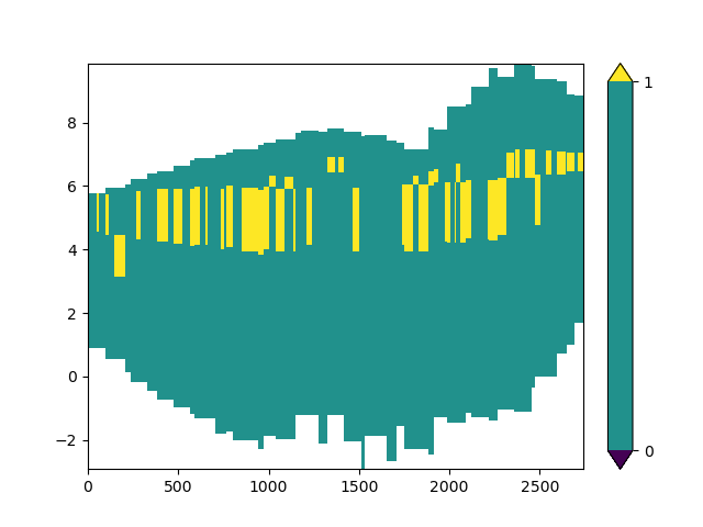
Now that we have selected our data we can plot it.
imod.visualize.cross_section(xsection_allocated, "viridis", [0, 1])
(<Figure size 640x480 with 2 Axes>, <Axes: >)
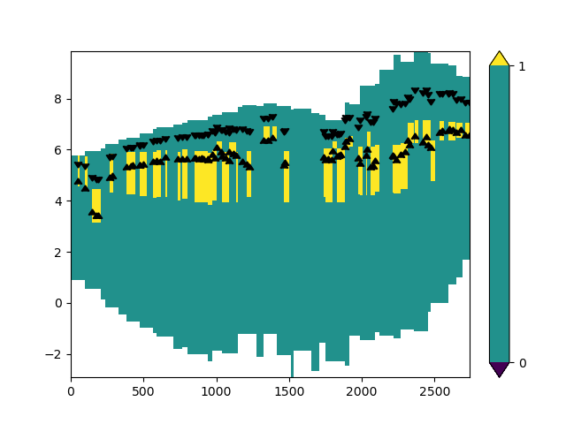
Let’s plot the locations of our river stages and bottom elevations.
import matplotlib.pyplot as plt

stage_line = imod.select.cross_section_linestring(planar_river["stage"], geometry)
stage_bottom = imod.select.cross_section_linestring(planar_river["bottom"], geometry)

fig, ax = plt.subplots()

imod.visualize.cross_section(xsection_allocated, "viridis", [0, 1], fig=fig, ax=ax)
x_line = stage_line["s"] + stage_line["ds"] / 2
ax.scatter(x_line, stage_line.values, marker=7, c="k")
ax.scatter(x_line, stage_bottom.values, marker=6, c="k")
<matplotlib.collections.PathCollection object at 0x0000019B26486510>
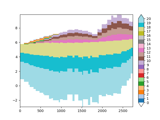
The above plot might look a bit off. Let’s plot the layer numbers, so that we can identify where model layers are located.
import xarray as xr

layer_grid = layer_model.layer * xr.ones_like(layer_model["top"])
layer_grid.coords["top"] = layer_model["top"]
layer_grid.coords["bottom"] = layer_model["bottom"]
xsection_layer_nr = imod.select.cross_section_linestring(layer_grid, geometry)

imod.visualize.cross_section(xsection_layer_nr, "tab20", np.arange(21))
ax.scatter(x_line, stage_line.values, marker=7, c="k")
ax.scatter(x_line, stage_bottom.values, marker=6, c="k")
<matplotlib.collections.PathCollection object at 0x0000019B1FAA6C30>
Overview allocation options#
There are multiple options available to allocate rivers. For a full
description of all options, see the documentation of
imod.prepare.ALLOCATION_OPTION(). We can print all possible options as
follows:
for option in ALLOCATION_OPTION:
    print(option.name)
stage_to_riv_bot
first_active_to_elevation
stage_to_riv_bot_drn_above
at_elevation
at_first_active
Let’s make plots for each option to visualize the effect of each choice.
# Create grid for plots
fig, axes = plt.subplots(3, 2, sharex=True, sharey=True, figsize=(11, 11))
axes = np.ravel(axes)

# The top left plot shows the elevation of the river bottom (upward triangle)
# and river stage (downward triangle).
ax = axes[0]
imod.visualize.cross_section(
    xsection_layer_nr,
    "tab20",
    np.arange(21),
    kwargs_colorbar={"plot_colorbar": False},
    fig=fig,
    ax=ax,
)
ax.scatter(x_line, stage_line.values, marker=7, c="k")
ax.scatter(x_line, stage_bottom.values, marker=6, c="k")
ax.set_title("stage and bottom elevation")

# Loop over allocation options, and plot the allocated cells as a polygon,
# using the "aquitard" feature of the cross_section plot.
for i, option in enumerate(ALLOCATION_OPTION, start=1):
    riv_allocated, _ = allocate_riv_cells(
        allocation_option=option,
        active=layer_model["idomain"] == 1,
        top=layer_model["top"],
        bottom=layer_model["bottom"],
        stage=planar_river["stage"],
        bottom_elevation=planar_river["bottom"],
    )
    riv_allocated.coords["top"] = layer_model["top"]
    riv_allocated.coords["bottom"] = layer_model["bottom"]

    xsection_allocated = imod.select.cross_section_linestring(riv_allocated, geometry)
    ax = axes[i]
    if (i % 2) == 0:
        kwargs_colorbar = {"plot_colorbar": False}
    else:
        kwargs_colorbar = {"plot_colorbar": True}
    kwargs_aquitards = {"edgecolor": "k", "facecolor": "grey"}
    imod.visualize.cross_section(
        xsection_layer_nr,
        "tab20",
        np.arange(21),
        aquitards=xsection_allocated,
        kwargs_aquitards=kwargs_aquitards,
        kwargs_colorbar=kwargs_colorbar,
        fig=fig,
        ax=ax,
    )
    ax.set_title(f"option: {option.name}")

# Enforce tight layout to remove whitespace inbetween plots.
plt.tight_layout()
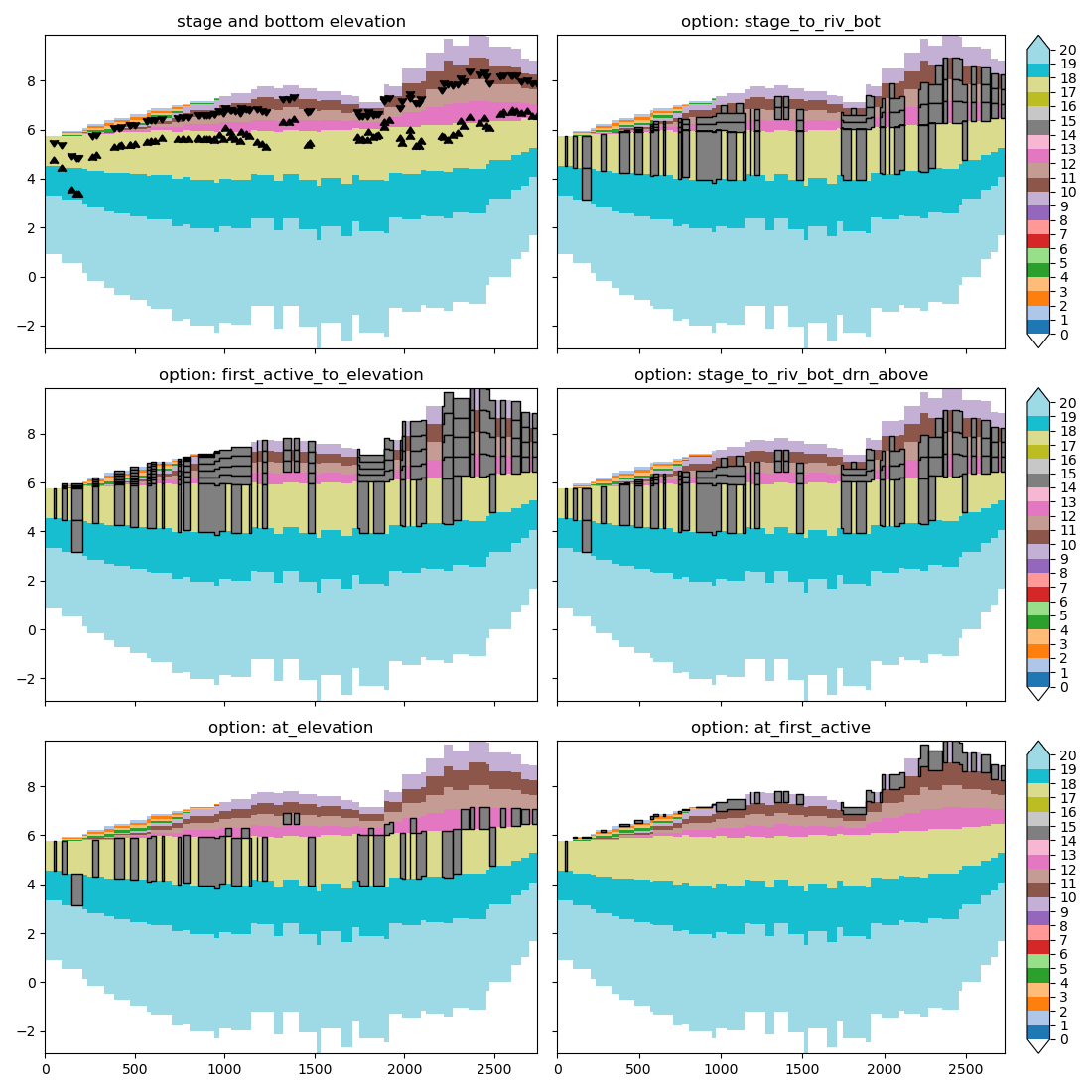
You can see the chosen option matters quite a lot. at_elevation allocates
cells in the model layer containing the river bottom elevation.
at_first_active allocates only at the first active model layer.
first_active_to_elevation allocates cells from first active model layer to
the model layer containing the river bottom elevation. stage_to_riv_bot
allocates cells from the model layer containing river stage up until the model
layer containing bottom elevation. Finally stage_to_riv_bot_drn_above
allocates river cells from the model layer containing river stage to the
model layer containing the river bottom elevation and allocates drain cells
from the first active model layer to the model layer containing the river
stage elevation. The allocated drain cells are not shown in the plot.
Distribute conductance#
Next, we’ll take a look at distributing conductances, as there are multiple ways to distribute conductances over layers. For example, it is possible to distribute conductances equally across layers, weighted by layer thickness, or by transmissivity.
from imod.prepare import DISTRIBUTING_OPTION, distribute_riv_conductance
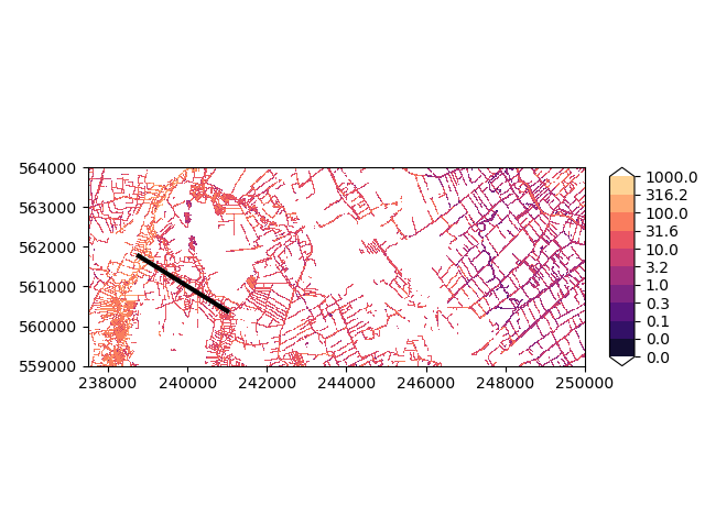
Here’s a map of how the conductances are distributed in our dataset.
imod.visualize.plot_map(
    planar_river["conductance"], "magma", np.logspace(-2, 3, 11), overlays
)
(<Figure size 640x480 with 2 Axes>, <Axes: >)
First compute the allocated river cells for stage to river bottom elevation
again. This time we’ll use the stage_to_riv_bot option.
riv_allocated, _ = allocate_riv_cells(
    allocation_option=ALLOCATION_OPTION.stage_to_riv_bot,
    active=layer_model["idomain"] == 1,
    top=layer_model["top"],
    bottom=layer_model["bottom"],
    stage=planar_river["stage"],
    bottom_elevation=planar_river["bottom"],
)

riv_allocated
Distribute river conductance over model layers. There are multiple options
available, which are fully described in
imod.prepare.DISTRIBUTING_OPTION(). We can print all possible options as
follows:
for option in DISTRIBUTING_OPTION:
    print(option.name)
by_corrected_transmissivity
by_corrected_thickness
equally
by_crosscut_thickness
by_layer_thickness
by_crosscut_transmissivity
by_conductivity
by_layer_transmissivity
To reduce duplicate code, we are going to store all input data in this dictionary which we can provide further as keyword arguments.
distributing_data = {
    "allocated": riv_allocated,
    "conductance": planar_river["conductance"],
    "top": layer_model["top"],
    "bottom": layer_model["bottom"],
    "k": layer_model["k"],
    "stage": planar_river["stage"],
    "bottom_elevation": planar_river["bottom"],
}
Let’s keep things simple first and distribute conductances across layers equally.
riv_conductance = distribute_riv_conductance(
    distributing_option=DISTRIBUTING_OPTION.by_layer_thickness, **distributing_data
)
riv_conductance.coords["top"] = layer_model["top"]
riv_conductance.coords["bottom"] = layer_model["bottom"]
Lets repeat the earlier process to produce a nice cross-section plot.
# Select the conductance over the cross section again.
xsection_distributed = imod.select.cross_section_linestring(riv_conductance, geometry)

fig, ax = plt.subplots()

# Plot grey background of active cells
is_active = ~np.isnan(xsection_distributed.coords["top"])
imod.visualize.cross_section(
    is_active,
    "Greys",
    [0, 1, 2, 3],
    kwargs_colorbar={"plot_colorbar": False},
    fig=fig,
    ax=ax,
)
# Plot conductances
imod.visualize.cross_section(
    xsection_distributed, "magma", np.logspace(-2, 3, 11), fig=fig, ax=ax
)
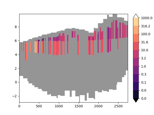
(<Figure size 640x480 with 2 Axes>, <Axes: >)
Let’s compare the results of all possible options visually. On the top left
we’ll plot the hydraulic conductivity, as we haven’t looked at that yet. The
other plots show the effects of different settings. Again, distributing
options are described in more detail in imod.prepare.DISTRIBUTING_OPTION()
fig, axes = plt.subplots(3, 3, figsize=[13, 11], sharex=True, sharey=True)
axes = np.ravel(axes)

k = distributing_data["k"].copy()
k.coords["top"] = layer_model["top"]
k.coords["bottom"] = layer_model["bottom"]

xsection_k = imod.select.cross_section_linestring(k, geometry)

ax = axes[0]
imod.visualize.cross_section(
    xsection_k,
    "magma",
    np.logspace(-2, 3, 11),
    kwargs_colorbar={"plot_colorbar": False},
    fig=fig,
    ax=ax,
)
ax.scatter(x_line, stage_line.values, marker=7, c="k")
ax.scatter(x_line, stage_bottom.values, marker=6, c="k")
ax.set_title("hydraulic conductivity")

for i, option in enumerate(DISTRIBUTING_OPTION, start=1):
    ax = axes[i]
    riv_conductance = distribute_riv_conductance(
        distributing_option=option, **distributing_data
    )
    riv_conductance.coords["top"] = layer_model["top"]
    riv_conductance.coords["bottom"] = layer_model["bottom"]

    xsection_distributed = imod.select.cross_section_linestring(
        riv_conductance, geometry
    )

    if (i % 3) == 2:
        kwargs_colorbar = {"plot_colorbar": True}
    else:
        kwargs_colorbar = {"plot_colorbar": False}

    # Plot grey background of active cells
    is_active = ~np.isnan(xsection_distributed.coords["top"])
    imod.visualize.cross_section(
        is_active,
        "Greys",
        [0, 1, 2, 3],
        kwargs_colorbar={"plot_colorbar": False},
        fig=fig,
        ax=ax,
    )
    # Plot conductances
    imod.visualize.cross_section(
        xsection_distributed,
        "magma",
        np.logspace(-2, 3, 11),
        kwargs_colorbar=kwargs_colorbar,
        fig=fig,
        ax=ax,
    )

    ax.set_title(f"option: {option.name}")

plt.tight_layout()
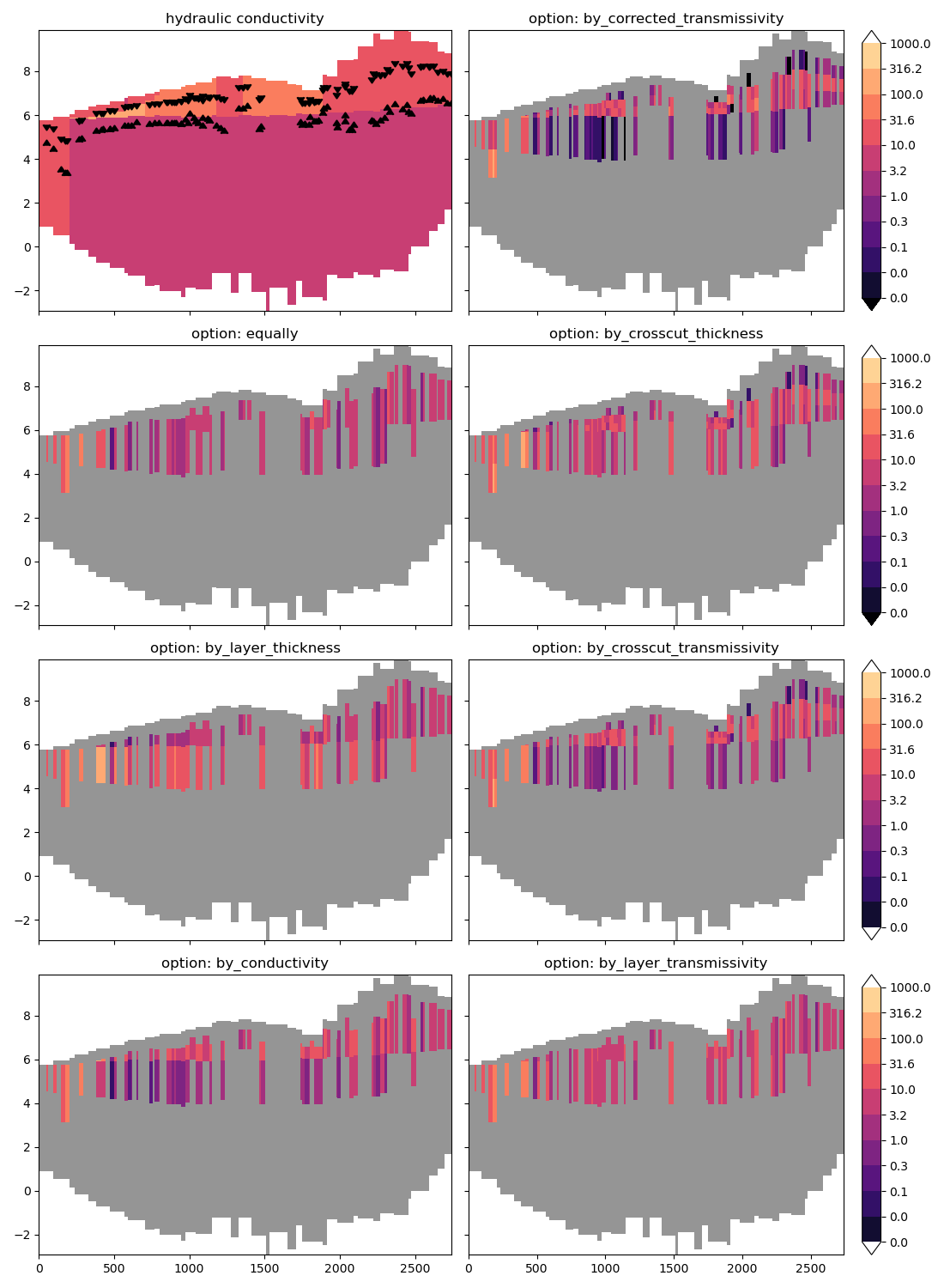
You can see quite some wildly varying conductances with depth. First, the most
simple algorithm equally keeps conductance constant with depth. Second,
correcting by_conductivity (hydraulic) decreases the conductance in the
deepest layer where rivers occur in the centre of the plot, as conductivity is
lower over there. Correcting by_layer_thickness, however, increases
conductance in this deep layer, as this is a thicker layer. These differences
even out when we correct by_layer_transmissivity (k * thickness). The
by_crosscut_thickness algorithm accounts for how far the river bottom
penetrates a layer. You can see this reduces conductance in the deep layer
compared to distributing by_layer_thickness.
by_crosscut_transmissivity uses the crosscut thickness instead of the
layer thickness and therefore shows a lower conductance in the deeper layer
compared to by_layer_transmissivity. Finally
by_corrected_transmissivity and by_corrected_thickness also correct
for the displacement of the midpoint over the length where crosscut
transmissivity is computed over ([layer top - river bottom]/2) compared to
the model cell centre. This further reduces the conductance in the deeper
layer.
MODFLOW 6 package#
The data created can now be used to create a MODFLOW 6 package. To construct 3D grids from planar grids for the stages, we can utilize xarrays broadcasting:
from imod.typing.grid import enforce_dim_order

riv_stage = planar_river["stage"].where(riv_allocated)
# Use this function to enforce the right dimension order for iMOD Python.
riv_stage = enforce_dim_order(riv_stage)

riv_stage
We can do the same for the river bottom and construct a river package. Note
that we use the previously distributed conductance which we assigned to the
variable riv_conductance.
riv_bottom = planar_river["bottom"].where(riv_allocated)
riv_bottom = enforce_dim_order(riv_bottom)

# Remove coordinates that were added for cross-section plots previously
riv_conductance = riv_conductance.drop_vars(["bottom", "top"])

riv = imod.mf6.River(
    stage=riv_stage, conductance=riv_conductance, bottom_elevation=riv_bottom
)

riv
Reallocate package#
The river package has a imod.mf6.River.reallocate() method which can be
used to reallocate the river package to a new model layer schematization. This
is convenient when you already have an existing model, but want to apply a
different allocation or distribution option to its river package. This saves
you from unpacking the right variables from the the DIS/DISV and NPF package,
aggregating the package data over layers and allocating and distributing the
conductance again. There are equivalent methods for the
imod.mf6.Drainage.reallocate(),
imod.mf6.GeneralHeadBoundary.reallocate(), and
imod.mf6.Recharge.reallocate().
dis = imod.mf6.StructuredDiscretization(
    top=layer_model["top"].sel(layer=1),
    bottom=layer_model["bottom"],
    idomain=layer_model["idomain"].astype(int),
)
npf = imod.mf6.NodePropertyFlow(icelltype=0, k=layer_model["k"])

riv_reallocated = riv.reallocate(
    dis, npf, allocation_option=ALLOCATION_OPTION.stage_to_riv_bot
)

riv_reallocated
The default allocation option and distribution option for the are set in the
imod.prepare.SimulationAllocationOptions and
imod.prepare.SimulationDistributingOptions. Let’s print the default
options to see what they are. First let’s start with the allocation options:
from dataclasses import asdict

from imod.prepare import SimulationAllocationOptions, SimulationDistributingOptions

print(asdict(SimulationAllocationOptions()))
{'drn': <ALLOCATION_OPTION.at_elevation: 2>, 'riv': <ALLOCATION_OPTION.stage_to_riv_bot: 0>, 'ghb': <ALLOCATION_OPTION.at_elevation: 2>, 'rch': <ALLOCATION_OPTION.at_first_active: 9>}
Now let’s print the distribution options:
print(asdict(SimulationDistributingOptions()))
{'drn': <DISTRIBUTING_OPTION.by_layer_transmissivity: 9>, 'riv': <DISTRIBUTING_OPTION.by_corrected_transmissivity: -1>, 'ghb': <DISTRIBUTING_OPTION.by_layer_transmissivity: 9>}
Total running time of the script: (0 minutes 11.938 seconds)