Tip
Example: Reading tiled raster data with different zoom levels#
This example will show how one can export raster dataset to individual tiles at differnt zoom levels and read the data via the DataCatalog.get_rasterdataset method.
[1]:
# Imports
from hydromt import raster, DataCatalog
from hydromt.log import setuplog
from os.path import join

logger = setuplog("tiling", log_level=20)

# get some elevation data from the data catalog
data_lib = "artifact_data"
data_cat = DataCatalog(data_lib, logger=logger)
source = "merit_hydro"
da0 = data_cat.get_rasterdataset(source, variables=["elevtn"])
da0.raster.shape
2024-04-25 17:22:00,970 - tiling - log - INFO - HydroMT version: 0.9.5.dev0
2024-04-25 17:22:00,996 - tiling - data_catalog - INFO - Reading data catalog archive artifact_data v0.0.8
2024-04-25 17:22:00,997 - tiling - data_catalog - INFO - Parsing data catalog from /home/runner/.hydromt_data/artifact_data/v0.0.8/data_catalog.yml
2024-04-25 17:22:01,043 - tiling - rasterdataset - INFO - Reading merit_hydro raster data from /home/runner/.hydromt_data/artifact_data/v0.0.8/merit_hydro/{variable}.tif
[1]:
(1920, 1680)
da0 is gridded data as an xarray.DataArray object. With HydroMT an xarray.DataArray has some extra functionality via .raster This extra functionality does include the ability to write a raster to a tile database (tiling).
Tiling raster with XYZ stucture#
First let’s have a look at the XYZ structure. an xarray.DataArray is simple written to a tile database in XYZ structure via .raster.to_xyz_tiles
[2]:
# Write the database in XYZ stucture
name = f"{source}_xyz"
root = join("tmpdir", name)
zoom_levels = [0, 1, 2, 3, 4]
da0.raster.to_xyz_tiles(
    root=root,
    tile_size=256,
    zoom_levels=zoom_levels,
    driver="GTiff",  # try also 'netcdf4'
    compress="deflate",
)
Tiles at zoomlevel 4 smaller than tile_size 256
The tiles in the ‘merit_hydro_xyz’ folder now contains the zoom_levels as defined above.
zoomlevel 0 is at the scale of the xarray.DataArray (one on one). zoomlevel 1 is downscaled by a factor 2 compared to zoomlevel 0. zoomlevel 3 is downscaled by a factor of 8 compared to zoomlevel 0, etc.
A mosaic is created per zoomlevel of these tiles in a .vrt file.
At last, a .yml file is produced which can be read by the DataCatalog of HydroMT.
Tiling raster with OSM stucture#
Now let’s have a look at tiling according to the OSM structure an xarray.DataArray is simple written to a tile database in OSM structure via .raster.to_slippy_tiles
[3]:
# Write the database in XYZ stucture
name_osm = f"{source}_osm"
root_osm = join("tmpdir", name_osm)
da0.raster.to_slippy_tiles(
    root=root_osm, driver="GTiff", reproj_method="average", write_vrt=True  # try also 'netcdf4'
)
The tiles in the ‘merit_hydro_OSM’ folder now contains all the zoom_levels from the minimal starting level (9) until the highest level (0).
Every tile, regardless of the zoomlevel, has a resolution of 256 by 256 pixels.
Zoomlevel 0 is at the scale of the entire world (one tile) and is the most downscaled. Zoomlevel 9 contains the highest resolution (most tiles) in regards to this tile database.
A mosaic is created per zoomlevel of these tiles in a .vrt file, if write_vrt=True (only applicable to nc and Gtiff files). At last, if write_vrt=True, a yaml file is produced which can be read by the DataCatalog of HydroMT.
Tiling raster for a webviewer#
Finally, let’s take a look at tiling of a raster dataset with its use being to view the data in a webviewer. This is easily done with the .raster.to_webviewer_tiles method.
[4]:
# Write the data in OSM structure, but to images!
from matplotlib import pyplot as plt


name_png = f"{source}_png"
root_png = join("tmpdir", name_png)
da0.raster.to_slippy_tiles(
    root=root_png,
)
Now that the images are created, let’s take a look at an individual tile.
[5]:
# View the data
from PIL import Image
import matplotlib.pyplot as plt

# Create a figure to show the image
fig = plt.figure()
fig.set_size_inches(2.5, 2.5)
ax = fig.add_subplot(111)
ax.set_position([0, 0, 1, 1])
ax.axis("off")

# Show the image
im = Image.open(join(root_png, "9", "273", "182.png"))
ax.imshow(im)
[5]:
<matplotlib.image.AxesImage at 0x7f36a5993f10>
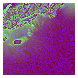
The image itself tends to look like an oil painting, but this is correct.
The colors for this image are determined so that they are correctly visually represented according to Terrarium Terrain RGB.
If one were to see what this would look like in e.g. QGIS, a local sever is needed. With python this is easily done with the command python -m http.server 8000 from the command line while within the folder where the tiles are located. In this case that would be ‘root_png’. In QGIS, make a new XYZ Tiles connection. For this new connection the URL becomes ‘http://localhost:8000/{z}/{x}/{y}.png’ and the interpolation is set to Terrarium Terrain RGB.
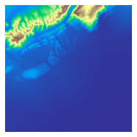
However, if the images are meant to be viewed as is, then a custom colormap can be defined to make them look nice!
Let’s make another dataset of png’s!
[6]:
from matplotlib import pyplot as plt


name_png_cmap = f"{source}_png_cmap"
root_png_cmap = join("tmpdir", name_png_cmap)
# let us define a nice color for a terrain image
da0.raster.to_slippy_tiles(
    root=root_png_cmap,
    cmap="terrain",
    norm=plt.Normalize(vmin=0, vmax=2000),
)
Now lets take a look at the improved standard visuals!
[7]:
# View the data
from PIL import Image
import matplotlib.pyplot as plt

# Create a figure to show the image
fig = plt.figure()
fig.set_size_inches(2.5, 2.5)
ax = fig.add_subplot(111)
ax.set_position([0, 0, 1, 1])
ax.axis("off")

# Show the image
im = Image.open(join(root_png_cmap, "9", "273", "182.png"))
ax.imshow(im)
[7]:
<matplotlib.image.AxesImage at 0x7f36a57d87d0>
Reading tiled raster data with zoom levels#
With DataCatalog.get_rasterdataset a raster (.vrt) can be retrieved. In case of a tile database it can be done for a certain zoomlevel. E.g.
[8]:
# Imports
from hydromt import DataCatalog

# Load the yml into a DataCatalog
data_catalog = DataCatalog(
    [join(root, f"{name}.yml"), join(root_osm, f"{name_osm}.yml")], logger=logger
)

# View the structure of the DataCatalog
data_catalog[name]
2024-04-25 17:22:17,324 - tiling - data_catalog - INFO - Parsing data catalog from tmpdir/merit_hydro_xyz/merit_hydro_xyz.yml
2024-04-25 17:22:17,326 - tiling - data_catalog - INFO - Parsing data catalog from tmpdir/merit_hydro_osm/merit_hydro_osm.yml
[8]:
crs: 4326
data_type: RasterDataset
driver: raster
nodata: -9999.0
path: /home/runner/work/hydromt/hydromt/docs/_examples/tmpdir/merit_hydro_xyz/merit_hydro_xyz_zl{zoom_level}.vrt
zoom_levels:
  0: 0.0008333333333333345
  1: 0.0016666666666666572
  2: 0.003333333333333316
  3: 0.006666666666666611
  4: 0.013333333333333244
[9]:
# For the osm dataset
data_catalog[name_osm]
[9]:
crs: 3857
data_type: RasterDataset
driver: raster
path: /home/runner/work/hydromt/hydromt/docs/_examples/tmpdir/merit_hydro_osm/lvl{zoom_level}.vrt
zoom_levels:
  7: 1222.9924525628203
  8: 611.4962262814097
  9: 305.74811314070485
  10: 152.87405657035288
  11: 76.43702828517598
[10]:
# without zoom_level the highest res data is fetched
da0 = data_catalog.get_rasterdataset(name)
da0.raster.shape
2024-04-25 17:22:17,338 - tiling - rasterdataset - INFO - Reading merit_hydro_xyz raster data from /home/runner/work/hydromt/hydromt/docs/_examples/tmpdir/merit_hydro_xyz/merit_hydro_xyz_zl{zoom_level}.vrt
[10]:
(2048, 1792)
[11]:
# And for OSM
da1 = data_catalog.get_rasterdataset(name_osm, zoom_level=11, geom=da0.raster.box)
da1.raster.shape
2024-04-25 17:22:17,365 - tiling - rasterdataset - INFO - Reading merit_hydro_osm raster data from /home/runner/work/hydromt/hydromt/docs/_examples/tmpdir/merit_hydro_osm/lvl{zoom_level}.vrt
2024-04-25 17:22:17,376 - tiling - io - WARNING - nodata value missing for /home/runner/work/hydromt/hydromt/docs/_examples/tmpdir/merit_hydro_osm/lvl11.vrt
[11]:
(3575, 2050)
[12]:
# Request a raster from the Datacatolog based on zoom resolution & unit
da = data_catalog.get_rasterdataset(name_osm, zoom_level=(1 / 600, "degree"))
da = data_catalog.get_rasterdataset(name_osm, zoom_level=(1e4, "meter"))
2024-04-25 17:22:17,393 - tiling - rasterdataset - INFO - Reading merit_hydro_osm raster data from /home/runner/work/hydromt/hydromt/docs/_examples/tmpdir/merit_hydro_osm/lvl{zoom_level}.vrt
2024-04-25 17:22:17,400 - tiling - io - WARNING - nodata value missing for /home/runner/work/hydromt/hydromt/docs/_examples/tmpdir/merit_hydro_osm/lvl10.vrt
2024-04-25 17:22:17,408 - tiling - rasterdataset - INFO - Reading merit_hydro_osm raster data from /home/runner/work/hydromt/hydromt/docs/_examples/tmpdir/merit_hydro_osm/lvl{zoom_level}.vrt
2024-04-25 17:22:17,414 - tiling - io - WARNING - nodata value missing for /home/runner/work/hydromt/hydromt/docs/_examples/tmpdir/merit_hydro_osm/lvl7.vrt
[13]:
# We can also directly request a specific zoom level
da = data_catalog.get_rasterdataset(name, zoom_level=zoom_levels[-1], geom=da0.raster.box)
print(da.raster.shape)
2024-04-25 17:22:17,426 - tiling - rasterdataset - INFO - Reading merit_hydro_xyz raster data from /home/runner/work/hydromt/hydromt/docs/_examples/tmpdir/merit_hydro_xyz/merit_hydro_xyz_zl{zoom_level}.vrt
(128, 112)
[14]:
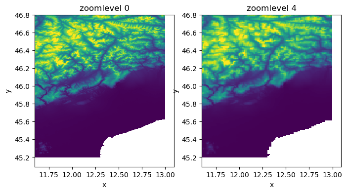
# View the data
import matplotlib.pyplot as plt

fig, (ax, ax1) = plt.subplots(1, 2, figsize=(8, 4))
da0.raster.mask_nodata().plot.imshow(ax=ax, vmin=0, vmax=2500, add_colorbar=False)
ax.set_title(f"zoomlevel {zoom_levels[0]}")
da.raster.mask_nodata().plot.imshow(ax=ax1, vmin=0, vmax=2500, add_colorbar=False)
ax1.set_title(f"zoomlevel {zoom_levels[-1]}")
[14]:
Text(0.5, 1.0, 'zoomlevel 4')
Caching tiled raster datasets#
Tiles of tiled rasterdatasets which are described by a .vrt file can be cached locally (starting from v0.7.0). The requested data tiles will by default be stored to ~/.hydromt_data.
[15]:
# set caching to True
# NOTE this can also be done at initialization of the DataCatalog
data_catalog.cache = True

# request some tiles based on bbox -> note the log messages
da0 = data_catalog.get_rasterdataset(name, bbox=[11.6, 45.3, 12.0, 46.0])
2024-04-25 17:22:17,972 - tiling - rasterdataset - INFO - Reading merit_hydro_xyz raster data from /home/runner/work/hydromt/hydromt/docs/_examples/tmpdir/merit_hydro_xyz/merit_hydro_xyz_zl{zoom_level}.vrt
2024-04-25 17:22:17,981 - tiling - caching - INFO - Downloading 56 tiles to /home/runner/.hydromt_data/merit_hydro_xyz/merit_hydro_xyz
[16]:
# if we run the same request again we will use the cached files (and download none)
da0 = data_catalog.get_rasterdataset(name, bbox=[11.6, 45.3, 12.0, 46.0])
2024-04-25 17:22:18,015 - tiling - rasterdataset - INFO - Reading merit_hydro_xyz raster data from /home/runner/work/hydromt/hydromt/docs/_examples/tmpdir/merit_hydro_xyz/merit_hydro_xyz_zl{zoom_level}.vrt
2024-04-25 17:22:18,019 - tiling - caching - INFO - Downloading 0 tiles to /home/runner/.hydromt_data/merit_hydro_xyz/merit_hydro_xyz