Tip
Example: Reading geospatial point time-series#
This example illustrates the how to read geospatial point time-series data here called GeoDataset, using the HydroMT DataCatalog with the vector and netcdf or zarr drivers.
[1]:
from pprint import pprint

import numpy as np

import hydromt
from hydromt import log

log.initialize_logging()
/home/runner/work/hydromt/hydromt/.pixi/envs/default/lib/python3.14/site-packages/tqdm/auto.py:21: TqdmWarning: IProgress not found. Please update jupyter and ipywidgets. See https://ipywidgets.readthedocs.io/en/stable/user_install.html
  from .autonotebook import tqdm as notebook_tqdm
2026-07-02 09:56:08,688 - hydromt - log - INFO - HydroMT version: 1.5.0.dev0
[2]:
# Download artifacts for the Piave basin
data_catalog = hydromt.DataCatalog(data_libs=["artifact_data=v1.0.0"])
2026-07-02 09:56:08,709 - hydromt.data_catalog.data_catalog - data_catalog - INFO - Reading data catalog artifact_data v1.0.0
2026-07-02 09:56:08,709 - hydromt.data_catalog.data_catalog - data_catalog - INFO - Parsing data catalog from /home/runner/.hydromt/artifact_data/v1.0.0/data_catalog.yml
Xarray Driver#
To read geospatial point time-series data and parse it into a xarray Dataset or DataArray we use the open_mfdataset() or the open_zarr() method. All options in the data catalog yaml file will be passed to to these methods.
As an example we will use the GTSM data dataset which is stored in Netcdf format.
[3]:
# inspect data source entry in data catalog yaml file
data_catalog.get_source("gtsmv3_eu_era5")
[3]:
GeoDatasetSource(name='gtsmv3_eu_era5', uri='gtsmv3_eu_era5.nc', data_adapter=GeoDatasetAdapter(unit_add={}, unit_mult={}, rename={}), driver=GeoDatasetXarrayDriver(filesystem=FSSpecFileSystem(protocol='file', storage_options={}), options=XarrayDriverOptions(preprocess=None, ext_override=None)), uri_resolver=ConventionResolver(filesystem=FSSpecFileSystem(protocol='file', storage_options={}), options={}), root='/home/runner/.hydromt/artifact_data/v1.0.0', version='3.0', provider=None, metadata=SourceMetadata(crs=<Geographic 2D CRS: EPSG:4326>
Name: WGS 84
Axis Info [ellipsoidal]:
- Lat[north]: Geodetic latitude (degree)
- Lon[east]: Geodetic longitude (degree)
Area of Use:
- name: World.
- bounds: (-180.0, -90.0, 180.0, 90.0)
Datum: World Geodetic System 1984 ensemble
- Ellipsoid: WGS 84
- Prime Meridian: Greenwich
, unit=None, extent={}, nodata=None, attrs={}, category='ocean', paper_doi='10.24381/cds.8c59054f', paper_ref='Copernicus Climate Change Service 2019', url='https://cds.climate.copernicus.eu/cdsapp#!/dataset/10.24381/cds.8c59054f?tab=overview', license='https://cds.climate.copernicus.eu/cdsapp/#!/terms/licence-to-use-copernicus-products'))
We can load any geospatial point time-series data using DataCatalog.get_geodataset(). Note that if we don’t provide any arguments it returns the full dataset with all data variables and for the full spatial domain. The result is per default returned as DataArray as the dataset consists of a single variable. To return a dataset use the single_var_as_array=False argument. Only the data coordinates and the time are actually
read, the data variables are still lazy Dask arrays.
[4]:
ds = data_catalog.get_geodataset("gtsmv3_eu_era5", single_var_as_array=False)
ds
2026-07-02 09:56:09,344 - hydromt.data_catalog.sources.data_source - data_source - INFO - Reading gtsmv3_eu_era5 GeoDataset data from /home/runner/.hydromt/artifact_data/v1.0.0/gtsmv3_eu_era5.nc
[4]:
<xarray.Dataset> Size: 323kB
Dimensions:      (time: 2016, stations: 19)
Coordinates:
  * time         (time) datetime64[ns] 16kB 2010-02-01 ... 2010-02-14T23:50:00
  * stations     (stations) int32 76B 13670 2798 2799 13775 ... 2791 2790 2789
    lon          (stations) float64 152B dask.array<chunksize=(19,), meta=np.ndarray>
    lat          (stations) float64 152B dask.array<chunksize=(19,), meta=np.ndarray>
    spatial_ref  int32 4B ...
Data variables:
    waterlevel   (time, stations) float64 306kB dask.array<chunksize=(2016, 19), meta=np.ndarray>
Attributes:
    crs:        4326
    category:   ocean
    paper_doi:  10.24381/cds.8c59054f
    paper_ref:  Copernicus Climate Change Service 2019
    url:        https://cds.climate.copernicus.eu/cdsapp#!/dataset/10.24381/c...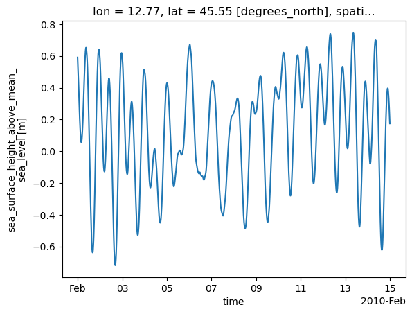
license: https://cds.climate.copernicus.eu/cdsapp/#!/terms/licence-to-...The data can be visualized with the DataArray.plot() xarray method. We show the evolution of the water level over time for a specific point location (station).
[5]:
ds.sel(stations=2791)["waterlevel"].plot()
[5]:
[<matplotlib.lines.Line2D at 0x7fd4a75e06e0>]
We can request a (spatial) subset data by providing additional variables and bbox / geom arguments. Note that these return less stations and less variables. In this example only spatial arguments are applied as only a single variable is available. The variables argument is especially useful if each variable of the dataset is saved in a separate file and the {variable} key is used in the path argument of the data source to limit which files are actually read. If a single variable
is requested a DataArray instead of a Dataset is returned unless the single_var_as_array argument is set to False (True by default).
[6]:
bbox = [12.50, 45.20, 12.80, 45.40]
ds_bbox = data_catalog.get_geodataset("gtsmv3_eu_era5", bbox=bbox)
ds_bbox
2026-07-02 09:56:09,926 - hydromt.data_catalog.sources.data_source - data_source - INFO - Reading gtsmv3_eu_era5 GeoDataset data from /home/runner/.hydromt/artifact_data/v1.0.0/gtsmv3_eu_era5.nc
[6]:
<xarray.DataArray 'waterlevel' (time: 2016, stations: 2)> Size: 32kB
dask.array<getitem, shape=(2016, 2), dtype=float64, chunksize=(2016, 2), chunktype=numpy.ndarray>
Coordinates:
  * time         (time) datetime64[ns] 16kB 2010-02-01 ... 2010-02-14T23:50:00
  * stations     (stations) int32 8B 13775 13723
    lon          (stations) float64 16B dask.array<chunksize=(2,), meta=np.ndarray>
    lat          (stations) float64 16B dask.array<chunksize=(2,), meta=np.ndarray>
    spatial_ref  int32 4B ...
Attributes:
    long_name:       sea_surface_height_above_mean_sea_level
    units:           m
    CDI_grid_type:   unstructured
    short_name:      waterlevel
    description:     Total water level resulting from the combination of baro...
    category:        ocean
    paper_doi:       10.24381/cds.8c59054f
    paper_ref:       Copernicus Climate Change Service 2019
    source_license:  https://cds.climate.copernicus.eu/cdsapp/#!/terms/licenc...
    source_url:      https://cds.climate.copernicus.eu/cdsapp#!/dataset/10.24...
source_version: GTSM v3.0With a Geodataset, you can also directly access the associated point geometries using its to_gdf() method. Multi-dimensional data (e.g. the time series) can be reduced using a statistical method such as the max.
[7]:
pprint(ds_bbox.vector.to_gdf(reducer=np.nanmax))
                           geometry  waterlevel
stations
13775     POINT (12.75879 45.24902)    0.703679
13723     POINT (12.50244 45.25635)    0.721433
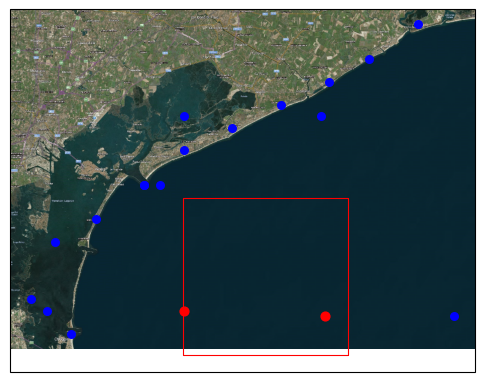
[8]:
# Plot
import cartopy.crs as ccrs
import cartopy.io.img_tiles as cimgt
import geopandas as gpd
import matplotlib.pyplot as plt
from shapely.geometry import box

proj = ccrs.PlateCarree()

fig = plt.figure(figsize=(6, 10))
ax = plt.subplot(projection=proj)

bbox = gpd.GeoDataFrame(geometry=[box(12.50, 45.20, 12.80, 45.40)], crs=4326)

ax.add_image(cimgt.QuadtreeTiles(), 12)
# Plot the points
ds.vector.to_gdf().plot(ax=ax, markersize=30, c="blue", zorder=2)
ds_bbox.vector.to_gdf().plot(ax=ax, markersize=40, c="red", zorder=2)
# Plot the bounding box
bbox.boundary.plot(ax=ax, color="red", linewidth=0.8)
[8]:
<GeoAxes: >
Vector driver#
To read vector data and parse it into a xarray.Dataset object we use the get_geodataset() method. Combined point locations (e.g. CSV or GeoJSON) data as well as text delimited time series (e.g. CSV) data are supported as file formats (see DataCatalog documentation). Both formats must contain an index and a crs has to be indicated in the .yml file. For demonstration we use dummy example data from the examples/data folder.
First load the data catalog of the corresponding example data geodataset_catalog.yml:
[9]:
geodata_catalog = hydromt.DataCatalog("data/geodataset_catalog.yml")
geodata_catalog.get_source("waterlevels_txt")
2026-07-02 09:56:12,934 - hydromt.data_catalog.data_catalog - data_catalog - INFO - Parsing data catalog from data/geodataset_catalog.yml
[9]:
GeoDatasetSource(name='waterlevels_txt', uri='stations.csv', data_adapter=GeoDatasetAdapter(unit_add={}, unit_mult={}, rename={'stations_data': 'waterlevel'}), driver=GeoDatasetVectorDriver(filesystem=FSSpecFileSystem(protocol='file', storage_options={}), options=XarrayDriverOptions(preprocess=None, ext_override=None, data_path='stations_data.csv')), uri_resolver=ConventionResolver(filesystem=FSSpecFileSystem(protocol='file', storage_options={}), options={}), root='data', version=None, provider=None, metadata=SourceMetadata(crs=<Geographic 2D CRS: EPSG:4326>
Name: WGS 84
Axis Info [ellipsoidal]:
- Lat[north]: Geodetic latitude (degree)
- Lon[east]: Geodetic longitude (degree)
Area of Use:
- name: World.
- bounds: (-180.0, -90.0, 180.0, 90.0)
Datum: World Geodetic System 1984 ensemble
- Ellipsoid: WGS 84
- Prime Meridian: Greenwich
, unit=None, extent={}, nodata=None, attrs={}, category=None))
We see here that our locations are defined in a data/stations.csv file and a data/stations_data.csv. Let’s check the content of these files before loading them with the get_geodataset method:
[10]:
import pandas as pd

print("Stations locations:")
df_stations = pd.read_csv("data/stations.csv")
pprint(df_stations)
Stations locations:
   stations         x         y
0      1001  12.50244  45.25635
1      1002  12.75879  45.24902
[11]:
print("Stations data:")
df_stations_data = pd.read_csv("data/stations_data.csv")
pprint(df_stations_data.head(3))
Stations data:
         time      1001      1002
0  2016-01-01  0.590860  0.591380
1  2016-01-02  0.565552  0.571342
2  2016-01-03  0.538679  0.549770
[12]:
ds = geodata_catalog.get_geodataset("waterlevels_txt", single_var_as_array=False)
ds
2026-07-02 09:56:12,955 - hydromt.data_catalog.sources.data_source - data_source - INFO - Reading waterlevels_txt GeoDataset data from /home/runner/work/hydromt/hydromt/docs/_examples/data/stations.csv
[12]:
<xarray.Dataset> Size: 48kB
Dimensions:      (time: 2016, stations: 2)
Coordinates:
  * time         (time) datetime64[ns] 16kB 2016-01-01 2016-01-02 ... 2021-07-08
  * stations     (stations) int64 16B 1001 1002
    geometry     (stations) object 16B dask.array<chunksize=(2,), meta=np.ndarray>
    spatial_ref  int64 8B 0
Data variables:
    waterlevel   (stations, time) float64 32kB dask.array<chunksize=(2, 2016), meta=np.ndarray>
Attributes:
    crs:      4326