Tip
Example: Reading 2D tabular data (DataFrame)#
This example illustrates the how to read 2D tabular data using the HydroMT DataCatalog with the csv driver.
[1]:
from hydromt import DataCatalog, log

log.initialize_logging()

data_catalog = DataCatalog("data/tabular_data_catalog.yml")
/home/runner/work/hydromt/hydromt/.pixi/envs/default/lib/python3.14/site-packages/tqdm/auto.py:21: TqdmWarning: IProgress not found. Please update jupyter and ipywidgets. See https://ipywidgets.readthedocs.io/en/stable/user_install.html
  from .autonotebook import tqdm as notebook_tqdm
2026-07-02 09:56:25,789 - hydromt - log - INFO - HydroMT version: 1.5.0.dev0
2026-07-02 09:56:25,790 - hydromt.data_catalog.data_catalog - data_catalog - INFO - Parsing data catalog from data/tabular_data_catalog.yml
Pandas driver#
time series data#
To read 2D tabular data from a comma-separated file (csv) and parse it into a pandas.DataFrame we use the pandas.read_csv(). Any driver_kwargs in the data catalog are passed to this method, e.g., parsing dates in the “time” colum and setting this as the index.
This works similarly for excel tables, but based on the pandas.read_excel() method.
For demonstration we use a dummy example timeseries data in csv.
[2]:
# inspect data source entry in data catalog yaml file
data_catalog.get_source("example_csv_data")
[2]:
DataFrameSource(name='example_csv_data', uri='example_csv_data.csv', data_adapter=DataFrameAdapter(unit_add={}, unit_mult={}, rename={}), driver=PandasDriver(filesystem=FSSpecFileSystem(protocol='file', storage_options={}), options=DriverOptions(parse_dates=True, index_col='time')), uri_resolver=ConventionResolver(filesystem=FSSpecFileSystem(protocol='file', storage_options={}), options={}), root='data', version=None, provider=None, metadata=SourceMetadata(crs=None, unit=None, extent={}, nodata=None, attrs={}, category=None))
We can load any 2D tabular data using DataCatalog.get_dataframe(). Note that if we don’t provide any arguments it returns the full dataframe.
[3]:
df = data_catalog.get_dataframe("example_csv_data")
df.head()
2026-07-02 09:56:25,819 - hydromt.data_catalog.sources.data_source - data_source - INFO - Reading example_csv_data DataFrame data from /home/runner/work/hydromt/hydromt/docs/_examples/data/example_csv_data.csv
[3]:
| col1 | col2 | |
|---|---|---|
| time | ||
| 2016-01-01 | 0.590860 | 0.591380 |
| 2016-01-02 | 0.565552 | 0.571342 |
| 2016-01-03 | 0.538679 | 0.549770 |
| 2016-01-04 | 0.511894 | 0.526932 |
| 2016-01-05 | 0.483989 | 0.502907 |
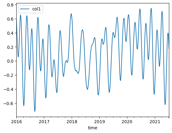
The data can be visualized with the .plot() pandas method.
[4]:
df.plot(y="col1")
[4]:
<Axes: xlabel='time'>
reclassification table#
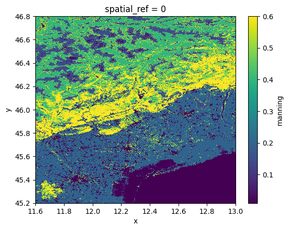
Another typical usecase for tabular data are reclassification tables to reclassify e.g. land use data to manning roughness. An example of this data is shown in the cells below. Note tha the values are not validated and likely too high!
[5]:
# read both the vito_reclass and artifact_data data catalogs
data_catalog = DataCatalog(["data/vito_reclass.yml", "artifact_data"])
data_catalog.get_source("vito_reclass")
2026-07-02 09:56:26,336 - hydromt.data_catalog.data_catalog - data_catalog - INFO - Parsing data catalog from data/vito_reclass.yml
2026-07-02 09:56:26,353 - hydromt.data_catalog.data_catalog - data_catalog - INFO - Reading data catalog artifact_data latest
2026-07-02 09:56:26,353 - hydromt.data_catalog.data_catalog - data_catalog - INFO - Parsing data catalog from /home/runner/.hydromt/artifact_data/v1.0.0/data_catalog.yml
[5]:
DataFrameSource(name='vito_reclass', uri='vito_reclass.csv', data_adapter=DataFrameAdapter(unit_add={}, unit_mult={}, rename={}), driver=PandasDriver(filesystem=FSSpecFileSystem(protocol='file', storage_options={}), options=DriverOptions(index_col=0)), uri_resolver=ConventionResolver(filesystem=FSSpecFileSystem(protocol='file', storage_options={}), options={}), root='data', version=None, provider=None, metadata=SourceMetadata(crs=None, unit=None, extent={}, nodata=None, attrs={}, category=None, notes='reclass table for manning values'))
[6]:
df = data_catalog.get_dataframe("vito_reclass")
df.head()
2026-07-02 09:56:26,970 - hydromt.data_catalog.sources.data_source - data_source - INFO - Reading vito_reclass DataFrame data from /home/runner/work/hydromt/hydromt/docs/_examples/data/vito_reclass.csv
[6]:
| description | landuse | manning | |
|---|---|---|---|
| vito | |||
| 0 | Unknown | 0 | -999.000 |
| 20 | Shrubs | 20 | 0.500 |
| 30 | Herbaceous vegetation | 30 | 0.150 |
| 40 | Cultivated and managed vegetation/agriculture ... | 40 | 0.200 |
| 50 | Urban / built up | 50 | 0.011 |
[7]:
da_lulc = data_catalog.get_rasterdataset("vito_2015")
da_man = da_lulc.raster.reclassify(df[["manning"]])
da_man["manning"].plot.imshow()
2026-07-02 09:56:26,980 - hydromt.data_catalog.sources.data_source - data_source - INFO - Reading vito_2015 RasterDataset data from /home/runner/.hydromt/artifact_data/latest/vito.tif
[7]:
<matplotlib.image.AxesImage at 0x7f226c4abe00>