Tip

For an interactive online version click here:

Example: Reading vector data

This example illustrates the how to read raster data using the HydroMT DataCatalog with the vector or vector_table drivers.

# import hydromt and setup logging
import geopandas as gpd
import pandas as pd
import hydromt
from hydromt.log import setuplog

logger = setuplog("read vector data", log_level=10)

2024-04-25 17:19:47,246 - read vector data - log - INFO - HydroMT version: 0.9.5.dev0

# Download artifacts for the Piave basin to `~/.hydromt_data/`.
data_catalog = hydromt.DataCatalog(logger=logger, data_libs=["artifact_data"])

2024-04-25 17:19:47,276 - read vector data - data_catalog - INFO - Reading data catalog archive artifact_data v0.0.8

2024-04-25 17:19:47,276 - read vector data - data_catalog - INFO - Parsing data catalog from /home/runner/.hydromt_data/artifact_data/v0.0.8/data_catalog.yml

Vector driver

To read vector data and parse it into a geopandas.GeoDataFrame object we use the geopandas.read_file method, see the geopandas documentation for details. Geopandas supports many file formats, see below. For large datasets we recommend using data formats which contain a spatial index, such as ‘GeoPackage (GPKG)’ or ‘FlatGeoBuf’ to speed up reading spatial subsets of the data.

# uncomment to see list of supported file formats
# import fiona
# print(list(fiona.supported_drivers.keys()))

Here we use a spatial subset of the Database of Global Administrative Areas (GADM) level 3 units.

# inspect data source entry in data catalog yaml file
data_catalog["gadm_level3"]

crs: 4326
data_type: GeoDataFrame
driver: vector
meta:
  category: geography
  notes: last downloaded 2020-10-19; license required for commercial use
  source_author: gadm
  source_license: https://gadm.org/license.html
  source_url: https://gadm.org/download_world.html
  source_version: 1.0
path: /home/runner/.hydromt_data/artifact_data/v0.0.8/gadm_level3.gpkg

We can load any GeoDataFrame using the get_geodataframe() method of the DataCatalog. Note that if we don’t provide any arguments it returns the full dataset with nine data variables and for the full spatial domain. Only the data coordinates are actually read, the data variables are still loaded lazy.

gdf = data_catalog.get_geodataframe("gadm_level3")
print(f"number of rows: {gdf.index.size}")
gdf.head()

2024-04-25 17:19:47,339 - read vector data - geodataframe - INFO - Reading gadm_level3 vector data from /home/runner/.hydromt_data/artifact_data/v0.0.8/gadm_level3.gpkg

number of rows: 509

	GID_0	NAME_0	GID_1	NAME_1	NL_NAME_1	GID_2	NAME_2	NL_NAME_2	GID_3	NAME_3	VARNAME_3	NL_NAME_3	TYPE_3	ENGTYPE_3	CC_3	HASC_3	geometry
0	ITA	Italy	ITA.17_1	Trentino-Alto Adige	None	ITA.17.2_1	Trento	None	ITA.17.2.143_1	Predazzo	None	None	Commune	Commune	None	IT.TN.PA	MULTIPOLYGON (((11.74692 46.30762, 11.74614 46...
1	ITA	Italy	ITA.17_1	Trentino-Alto Adige	None	ITA.17.2_1	Trento	None	ITA.17.2.115_1	Moena	None	None	Commune	Commune	None	IT.TN.MN	MULTIPOLYGON (((11.82119 46.37751, 11.82013 46...
2	ITA	Italy	ITA.17_1	Trentino-Alto Adige	None	ITA.17.2_1	Trento	None	ITA.17.2.214_1	Vigo Di Fassa	None	None	Commune	Commune	None	IT.TN.VD	MULTIPOLYGON (((11.62028 46.43951, 11.62063 46...
3	ITA	Italy	ITA.17_1	Trentino-Alto Adige	None	ITA.17.2_1	Trento	None	ITA.17.2.36_1	Canal San Bovo	None	None	Commune	Commune	None	IT.TN.CB	MULTIPOLYGON (((11.75179 46.10603, 11.75210 46...
4	ITA	Italy	ITA.17_1	Trentino-Alto Adige	None	ITA.17.2_1	Trento	None	ITA.17.2.141_1	Pozza Di Fassa	None	None	Commune	Commune	None	IT.TN.PF	MULTIPOLYGON (((11.70521 46.40100, 11.70519 46...

We can request a (spatial) subset data by providing additional variables and bbox / geom arguments. Note that this returns less polygons (rows) and only two columns with attribute data,

gdf_subset = data_catalog.get_geodataframe(
    "gadm_level3", bbox=gdf[:5].total_bounds, variables=["GID_0", "NAME_3"]
)
print(f"number of rows: {gdf_subset.index.size}")
gdf_subset.head()

2024-04-25 17:19:47,546 - read vector data - geodataframe - INFO - Reading gadm_level3 vector data from /home/runner/.hydromt_data/artifact_data/v0.0.8/gadm_level3.gpkg

2024-04-25 17:19:47,571 - read vector data - geodataframe - DEBUG - Clip intersects [11.557, 46.096, 11.851, 46.477] (EPSG:4326)

number of rows: 28

	GID_0	NAME_3	geometry
0	ITA	Tonadico	MULTIPOLYGON (((11.84245 46.30723, 11.83778 46...
1	ITA	Siror	MULTIPOLYGON (((11.86518 46.27297, 11.86086 46...
2	ITA	Ziano Di Fiemme	MULTIPOLYGON (((11.55856 46.32783, 11.56022 46...
3	ITA	Predazzo	MULTIPOLYGON (((11.74692 46.30762, 11.74614 46...
4	ITA	Canale d' Agordo	MULTIPOLYGON (((11.86518 46.27297, 11.86392 46...

Vector_table driver

To read point vector data from a table (csv, xls or xlsx) we use the open_vector_from_table method.

# create example point CSV data with funny `x` coordinate name and additional column
import numpy as np
import pandas as pd

fn = "tmpdir/xy.csv"
df = pd.DataFrame(
    columns=["x_centroid", "y"],
    data=np.vstack([gdf_subset.centroid.x, gdf_subset.centroid.y]).T,
)
df["name"] = gdf_subset["NAME_3"]
df.to_csv(fn)  # write to file
df.head()

	x_centroid	y	name
0	11.838395	46.266421	Tonadico
1	11.790629	46.250124	Siror
2	11.583526	46.271041	Ziano Di Fiemme
3	11.644162	46.313247	Predazzo
4	11.885507	46.328140	Canale d' Agordo

# Create data source entry for the data catalog for the new csv data
# NOTE that we add specify the name of the x coordinate with the `x_dim` argument, while the y coordinate is understood by HydroMT.
data_source = {
    "GADM_level3_centroids": {
        "path": fn,
        "data_type": "GeoDataFrame",
        "driver": "vector_table",
        "crs": 4326,
        "driver_kwargs": {"x_dim": "x_centroid"},
    }
}
data_catalog.from_dict(data_source)
data_catalog["GADM_level3_centroids"]

crs: 4326
data_type: GeoDataFrame
driver: vector_table
driver_kwargs:
  x_dim: x_centroid
path: /home/runner/work/hydromt/hydromt/docs/_examples/tmpdir/xy.csv

# we can then read the data back as a GeoDataFrame
gdf_centroid = data_catalog.get_geodataframe("GADM_level3_centroids")
print(f"CRS: {gdf_centroid.crs}")
gdf_centroid.head()

2024-04-25 17:19:47,822 - read vector data - geodataframe - INFO - Reading GADM_level3_centroids vector_table data from /home/runner/work/hydromt/hydromt/docs/_examples/tmpdir/xy.csv

CRS: EPSG:4326

	name	geometry
0	Tonadico	POINT (11.83840 46.26642)
1	Siror	POINT (11.79063 46.25012)
2	Ziano Di Fiemme	POINT (11.58353 46.27104)
3	Predazzo	POINT (11.64416 46.31325)
4	Canale d' Agordo	POINT (11.88551 46.32814)

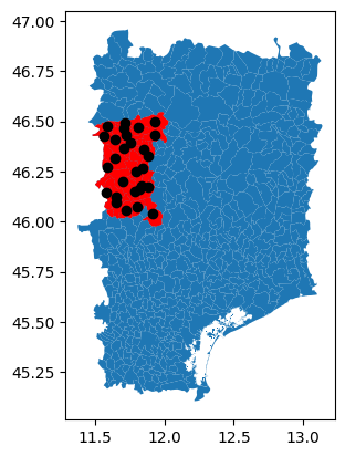
Visualize vector data

The data can be visualized with the .plot() geopandas method. In an interactive environment you can also try the .explore() method

# m = gdf.explore(width='20%', height='50%')
# gdf_subset.explore(m=m, color='red')  # subset in red
# m

ax = gdf.plot()
gdf_subset.plot(ax=ax, color="red")
gdf_centroid.plot(ax=ax, color="k")

<Axes: >