Tip
Example: Reading vector data#
This example illustrates the how to read raster data using the HydroMT DataCatalog with the vector or vector_table drivers.
[1]:
# import hydromt and setup logging
import geopandas as gpd
import pandas as pd
import hydromt
from hydromt.log import setuplog

logger = setuplog("read vector data", log_level=10)
2024-02-08 10:42:45,319 - read vector data - log - INFO - HydroMT version: 0.9.3
[2]:
# Download artifacts for the Piave basin to `~/.hydromt_data/`.
data_catalog = hydromt.DataCatalog(logger=logger, data_libs=["artifact_data"])
2024-02-08 10:42:45,347 - read vector data - data_catalog - INFO - Reading data catalog archive artifact_data v0.0.8
2024-02-08 10:42:45,348 - read vector data - data_catalog - INFO - Parsing data catalog from /home/runner/.hydromt_data/artifact_data/v0.0.8/data_catalog.yml
Vector driver#
To read vector data and parse it into a geopandas.GeoDataFrame object we use the geopandas.read_file method, see the geopandas documentation for details. Geopandas supports many file formats, see below. For large datasets we recommend using data formats which contain a spatial index, such as ‘GeoPackage (GPKG)’ or ‘FlatGeoBuf’ to speed up reading spatial subsets of the data.
[3]:
# uncomment to see list of supported file formats
# import fiona
# print(list(fiona.supported_drivers.keys()))
Here we use a spatial subset of the Database of Global Administrative Areas (GADM) level 3 units.
[4]:
# inspect data source entry in data catalog yaml file
data_catalog["gadm_level3"]
[4]:
crs: 4326
data_type: GeoDataFrame
driver: vector
meta:
  category: geography
  notes: last downloaded 2020-10-19; license required for commercial use
  source_author: gadm
  source_license: https://gadm.org/license.html
  source_url: https://gadm.org/download_world.html
  source_version: 1.0
path: /home/runner/.hydromt_data/artifact_data/v0.0.8/gadm_level3.gpkg
We can load any GeoDataFrame using the get_geodataframe() method of the DataCatalog. Note that if we don’t provide any arguments it returns the full dataset with nine data variables and for the full spatial domain. Only the data coordinates are actually read, the data variables are still loaded lazy.
[5]:
gdf = data_catalog.get_geodataframe("gadm_level3")
print(f"number of rows: {gdf.index.size}")
gdf.head()
2024-02-08 10:42:45,411 - read vector data - geodataframe - INFO - Reading gadm_level3 vector data from /home/runner/.hydromt_data/artifact_data/v0.0.8/gadm_level3.gpkg
number of rows: 509
[5]:
| GID_0 | NAME_0 | GID_1 | NAME_1 | NL_NAME_1 | GID_2 | NAME_2 | NL_NAME_2 | GID_3 | NAME_3 | VARNAME_3 | NL_NAME_3 | TYPE_3 | ENGTYPE_3 | CC_3 | HASC_3 | geometry | |
|---|---|---|---|---|---|---|---|---|---|---|---|---|---|---|---|---|---|
| 0 | ITA | Italy | ITA.17_1 | Trentino-Alto Adige | None | ITA.17.2_1 | Trento | None | ITA.17.2.143_1 | Predazzo | None | None | Commune | Commune | None | IT.TN.PA | MULTIPOLYGON (((11.74692 46.30762, 11.74614 46... |
| 1 | ITA | Italy | ITA.17_1 | Trentino-Alto Adige | None | ITA.17.2_1 | Trento | None | ITA.17.2.115_1 | Moena | None | None | Commune | Commune | None | IT.TN.MN | MULTIPOLYGON (((11.82119 46.37751, 11.82013 46... |
| 2 | ITA | Italy | ITA.17_1 | Trentino-Alto Adige | None | ITA.17.2_1 | Trento | None | ITA.17.2.214_1 | Vigo Di Fassa | None | None | Commune | Commune | None | IT.TN.VD | MULTIPOLYGON (((11.62028 46.43951, 11.62063 46... |
| 3 | ITA | Italy | ITA.17_1 | Trentino-Alto Adige | None | ITA.17.2_1 | Trento | None | ITA.17.2.36_1 | Canal San Bovo | None | None | Commune | Commune | None | IT.TN.CB | MULTIPOLYGON (((11.75179 46.10603, 11.75210 46... |
| 4 | ITA | Italy | ITA.17_1 | Trentino-Alto Adige | None | ITA.17.2_1 | Trento | None | ITA.17.2.141_1 | Pozza Di Fassa | None | None | Commune | Commune | None | IT.TN.PF | MULTIPOLYGON (((11.70521 46.40100, 11.70519 46... |
We can request a (spatial) subset data by providing additional variables and bbox / geom arguments. Note that this returns less polygons (rows) and only two columns with attribute data,
[6]:
gdf_subset = data_catalog.get_geodataframe(
    "gadm_level3", bbox=gdf[:5].total_bounds, variables=["GID_0", "NAME_3"]
)
print(f"number of rows: {gdf_subset.index.size}")
gdf_subset.head()
2024-02-08 10:42:45,611 - read vector data - geodataframe - INFO - Reading gadm_level3 vector data from /home/runner/.hydromt_data/artifact_data/v0.0.8/gadm_level3.gpkg
2024-02-08 10:42:45,791 - read vector data - geodataframe - DEBUG - Clip intersects [11.557, 46.096, 11.851, 46.477] (EPSG:4326)
number of rows: 28
[6]:
| GID_0 | NAME_3 | geometry | |
|---|---|---|---|
| 0 | ITA | Predazzo | MULTIPOLYGON (((11.74692 46.30762, 11.74614 46... |
| 1 | ITA | Moena | MULTIPOLYGON (((11.82119 46.37751, 11.82013 46... |
| 2 | ITA | Vigo Di Fassa | MULTIPOLYGON (((11.62028 46.43951, 11.62063 46... |
| 3 | ITA | Canal San Bovo | MULTIPOLYGON (((11.75179 46.10603, 11.75210 46... |
| 4 | ITA | Pozza Di Fassa | MULTIPOLYGON (((11.70521 46.40100, 11.70519 46... |
Vector_table driver#
To read point vector data from a table (csv, xls or xlsx) we use the open_vector_from_table method.
[7]:
# create example point CSV data with funny `x` coordinate name and additional column
import numpy as np
import pandas as pd

fn = "tmpdir/xy.csv"
df = pd.DataFrame(
    columns=["x_centroid", "y"],
    data=np.vstack([gdf_subset.centroid.x, gdf_subset.centroid.y]).T,
)
df["name"] = gdf_subset["NAME_3"]
df.to_csv(fn)  # write to file
df.head()
[7]:
| x_centroid | y | name | |
|---|---|---|---|
| 0 | 11.644162 | 46.313247 | Predazzo |
| 1 | 11.706954 | 46.365224 | Moena |
| 2 | 11.644298 | 46.411040 | Vigo Di Fassa |
| 3 | 11.700786 | 46.200499 | Canal San Bovo |
| 4 | 11.725591 | 46.429657 | Pozza Di Fassa |
[8]:
# Create data source entry for the data catalog for the new csv data
# NOTE that we add specify the name of the x coordinate with the `x_dim` argument, while the y coordinate is understood by HydroMT.
data_source = {
    "GADM_level3_centroids": {
        "path": fn,
        "data_type": "GeoDataFrame",
        "driver": "vector_table",
        "crs": 4326,
        "driver_kwargs": {"x_dim": "x_centroid"},
    }
}
data_catalog.from_dict(data_source)
data_catalog["GADM_level3_centroids"]
[8]:
crs: 4326
data_type: GeoDataFrame
driver: vector_table
driver_kwargs:
  x_dim: x_centroid
path: /home/runner/work/hydromt/hydromt/docs/_examples/tmpdir/xy.csv
[9]:
# we can then read the data back as a GeoDataFrame
gdf_centroid = data_catalog.get_geodataframe("GADM_level3_centroids")
print(f"CRS: {gdf_centroid.crs}")
gdf_centroid.head()
2024-02-08 10:42:46,002 - read vector data - geodataframe - INFO - Reading GADM_level3_centroids vector_table data from /home/runner/work/hydromt/hydromt/docs/_examples/tmpdir/xy.csv
CRS: EPSG:4326
[9]:
| name | geometry | |
|---|---|---|
| 0 | Predazzo | POINT (11.64416 46.31325) |
| 1 | Moena | POINT (11.70695 46.36522) |
| 2 | Vigo Di Fassa | POINT (11.64430 46.41104) |
| 3 | Canal San Bovo | POINT (11.70079 46.20050) |
| 4 | Pozza Di Fassa | POINT (11.72559 46.42966) |
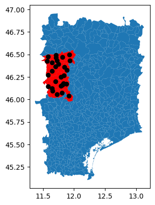
Visualize vector data#
The data can be visualized with the .plot() geopandas method. In an interactive environment you can also try the .explore() method
[10]:
# m = gdf.explore(width='20%', height='50%')
# gdf_subset.explore(m=m, color='red')  # subset in red
# m

ax = gdf.plot()
gdf_subset.plot(ax=ax, color="red")
gdf_centroid.plot(ax=ax, color="k")
[10]:
<Axes: >