Tip
Example: Preparing a data catalog#
This example illustrates the how to prepare your own HydroMT DataCatalog to reference your own data sources and start using then within HydroMT, see user guide.
[1]:
# import python libraries
import os
from pprint import pprint

import geopandas as gpd
import matplotlib.pyplot as plt
import pandas as pd
import rioxarray  # noqa
import xarray as xr

import hydromt
from hydromt import log

log.initialize_logging()
/home/runner/work/hydromt/hydromt/.pixi/envs/default/lib/python3.14/site-packages/tqdm/auto.py:21: TqdmWarning: IProgress not found. Please update jupyter and ipywidgets. See https://ipywidgets.readthedocs.io/en/stable/user_install.html
  from .autonotebook import tqdm as notebook_tqdm
2026-07-02 09:56:00,634 - hydromt - log - INFO - HydroMT version: 1.5.0.dev0
The steps to use your own data within HydroMT are in brief:
Have your (local) dataset ready in one of the supported raster (tif, ascii, netcdf, zarr…), vector (shp, geojson, gpkg…) or geospatial time-series (netcdf, csv…) format.
Create your own yaml file with a reference to your prepared dataset and properties (path, data_type, driver, etc.) following the HydroMT data conventions. For this step, you can also start from an existing pre-defined catalog or use it for inspiration.
The existing pre-defined catalog are:
[2]:
# this download the artifact_data archive v1.0.0
data_catalog = hydromt.DataCatalog(data_libs=["artifact_data=v1.0.0"])
pprint(data_catalog.predefined_catalogs)
2026-07-02 09:56:00,655 - hydromt.data_catalog.data_catalog - data_catalog - INFO - Reading data catalog artifact_data v1.0.0
2026-07-02 09:56:00,655 - hydromt.data_catalog.data_catalog - data_catalog - INFO - Parsing data catalog from /home/runner/.hydromt/artifact_data/v1.0.0/data_catalog.yml
{'artifact_data': <hydromt.data_catalog.predefined_catalog.ArtifactDataCatalog object at 0x7f5339d9ae40>,
 'aws_data': <hydromt.data_catalog.predefined_catalog.AWSDataCatalog object at 0x7f5339d9af90>,
 'deltares_data': <hydromt.data_catalog.predefined_catalog.DeltaresDataCatalog object at 0x7f5339d9a510>,
 'earthdatahub_data': <hydromt.data_catalog.predefined_catalog.EarthDataHubDataCatalog object at 0x7f5339d9b230>,
 'gcs_cmip6_data': <hydromt.data_catalog.predefined_catalog.GCSCMIP6DataCatalog object at 0x7f5339d9b0e0>}
In this notebook, we will see how we can create a data catalog for several type of input data. For this we have prepared several type of data that we will catalogue, let’s see which data we have available:
[3]:
# the artifact data is stored in the following location
root = os.path.join(data_catalog._cache_dir, "artifact_data", "v1.0.0")
# let's print some of the file that are there
for item in os.listdir(root)[-10:]:
    print(item)
merit_hydro
dtu10mdt_egm96.tif
eobs_orography.nc
data.tar.gz
koppen_geiger.tif
era5.nc
chirps_global.nc
grwl_tindex.gpkg
guf_bld_2012.tif
grdc.csv
RasterDataset from raster file#
The first file we will use is a ‘simple’ raster file in a tif format: vito.tif. This file contains a landuse classification raster. The first thing to do before adding a new file to a data catalog is to get to know what is inside of our file mainly:
location of the file:
path.type of data:
data_type.RasterDatasetfor gridded data,GeoDataFramefor vector data,GeoDatasetfor point timeseries andDataFramefor tabular data.file format:
driver. The file format impacts the driver or python function that will be used to open the data. Eitherraster,raster_tindex,netcdf,zarr,vector,vector_table.crs:
crs. Coordinate sytem of the data. Optional as it is usually encoded in the data itself.variables and their properties:
rename,unit_mult,unit_add. Looking at the variables in the input data and what are their names and units so that we can convert them to the HydroMT data conventions.
There are more arguments or properties to look for that are explained in more detailed in the documentation. To discover our data we can either use GIS software like QGIS or GDAL or just use python directly to try and open the data.
Let’s open our vito.tif file with xarray and rioxarray:
[4]:
da = xr.open_dataarray(os.path.join(root, "vito.tif"))
pprint(da)
print(f"CRS: {da.raster.crs}")
da.plot()
<xarray.DataArray 'band_data' (band: 1, y: 1613, x: 1412)> Size: 9MB
[2277556 values with dtype=float32]
Coordinates:
  * band         (band) int64 8B 1
  * y            (y) float64 13kB 46.8 46.8 46.8 46.8 ... 45.2 45.2 45.2 45.2
  * x            (x) float64 11kB 11.6 11.6 11.6 11.6 ... 13.0 13.0 13.0 13.0
    spatial_ref  int64 8B ...
Attributes:
    AREA_OR_POINT:  Area
CRS: GEOGCS["WGS 84",DATUM["WGS_1984",SPHEROID["WGS 84",6378137,298.257223563,AUTHORITY["EPSG","7030"]],AUTHORITY["EPSG","6326"]],PRIMEM["Greenwich",0,AUTHORITY["EPSG","8901"]],UNIT["degree",0.0174532925199433,AUTHORITY["EPSG","9122"]],AXIS["Latitude",NORTH],AXIS["Longitude",EAST],AUTHORITY["EPSG","4326"]]
[4]:
<matplotlib.collections.QuadMesh at 0x7f5339ba81a0>
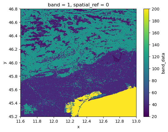
What we see is that we have a simple raster with landuse data in crs 4326. Let’s translate what we know into a data catalog.
[5]:
yml_str = f"""
meta:
  roots:
    - {root}

vito:
    uri: vito.tif
    data_type: RasterDataset
    driver:
      name: rasterio
    metadata:
      crs: 4326
"""
yaml_path = "tmpdir/vito.yml"
with open(yaml_path, mode="w") as f:
    f.write(yml_str)
And let’s now see if HydroMT can properly read the file from the data catalog we prepared:
[6]:
data_catalog = hydromt.DataCatalog(data_libs=[yaml_path])
da = data_catalog.get_rasterdataset("vito")
da
2026-07-02 09:56:02,909 - hydromt.data_catalog.data_catalog - data_catalog - INFO - Parsing data catalog from tmpdir/vito.yml
2026-07-02 09:56:02,912 - hydromt.data_catalog.sources.data_source - data_source - INFO - Reading vito RasterDataset data from /home/runner/.hydromt/artifact_data/v1.0.0/vito.tif
[6]:
<xarray.DataArray 'vito' (y: 1613, x: 1412)> Size: 2MB
[2277556 values with dtype=uint8]
Coordinates:
  * y            (y) float64 13kB 46.8 46.8 46.8 46.8 ... 45.2 45.2 45.2 45.2
  * x            (x) float64 11kB 11.6 11.6 11.6 11.6 ... 13.0 13.0 13.0 13.0
    spatial_ref  int64 8B 0
Attributes:
    AREA_OR_POINT:  Area
    _FillValue:     255
source_file: vito.tifRasterDataset from several raster files#
The second file we will add is the merit_hydro which consists of elevation and elevation-derived variables stored in several tif files for each variable. Let’s see what are their names.
[7]:
folder_name = os.path.join(root, "merit_hydro")
# let's see which files are there
for path, _, files in os.walk(folder_name):
    print(path)
    for name in files:
        print(f" - {name}")
/home/runner/.hydromt/artifact_data/v1.0.0/merit_hydro
 - elevtn.tif
 - flwdir.tif
 - lndslp.tif
 - rivwth.tif
 - upgrid.tif
 - hnd.tif
 - basins.tif
 - strord.tif
 - uparea.tif
We have here 9 files. When reading tif files, the name of the file is used as the variable name. HydroMT uses data conventions to ensure that certain variables should have the same name and units to be used in automatically in the workflows. For example elevation data should be called elevtn with unit in [m asl]. Check the data conventions and see if you need to rename or change units with unit_add and unit_mult for this dataset
in the data catalog.
Here all names and units are correct, so we just show an example were we rename the hnd variable.
[8]:
yml_str = f"""
meta:
  roots:
  - {root}

merit_hydro:
  data_type: RasterDataset
  driver:
    name: rasterio
    options:
      chunks:
        x: 6000
        y: 6000
  data_adapter:
    rename:
      hnd: height_above_nearest_drain
  uri: merit_hydro/*.tif
"""
# overwrite data catalog
data_lib = "tmpdir/merit_hydro.yml"
with open(data_lib, mode="w") as f:
    f.write(yml_str)
[9]:
data_catalog.from_yml(data_lib)  # add a yaml file to the data catalog
print(data_catalog.sources.keys())
ds = data_catalog.get_rasterdataset("merit_hydro")
ds
2026-07-02 09:56:02,941 - hydromt.data_catalog.data_catalog - data_catalog - INFO - Parsing data catalog from tmpdir/merit_hydro.yml
dict_keys(['vito', 'merit_hydro'])
2026-07-02 09:56:02,944 - hydromt.data_catalog.sources.data_source - data_source - INFO - Reading merit_hydro RasterDataset data from /home/runner/.hydromt/artifact_data/v1.0.0/merit_hydro/*.tif
[9]:
<xarray.Dataset> Size: 97MB
Dimensions:                     (x: 1680, y: 1920)
Coordinates:
  * x                           (x) float64 13kB 11.6 11.6 11.6 ... 13.0 13.0
  * y                           (y) float64 15kB 46.8 46.8 46.8 ... 45.2 45.2
    spatial_ref                 int64 8B 0
Data variables:
    flwdir                      (y, x) uint8 3MB dask.array<chunksize=(1920, 1680), meta=np.ndarray>
    upgrid                      (y, x) int32 13MB dask.array<chunksize=(1920, 1680), meta=np.ndarray>
    rivwth                      (y, x) float32 13MB dask.array<chunksize=(1920, 1680), meta=np.ndarray>
    strord                      (y, x) uint8 3MB dask.array<chunksize=(1920, 1680), meta=np.ndarray>
    uparea                      (y, x) float32 13MB dask.array<chunksize=(1920, 1680), meta=np.ndarray>
    basins                      (y, x) uint32 13MB dask.array<chunksize=(1920, 1680), meta=np.ndarray>
    elevtn                      (y, x) float32 13MB dask.array<chunksize=(1920, 1680), meta=np.ndarray>
    height_above_nearest_drain  (y, x) float32 13MB dask.array<chunksize=(1920, 1680), meta=np.ndarray>
lndslp (y, x) float32 13MB dask.array<chunksize=(1920, 1680), meta=np.ndarray>In the path, the filenames can be further specified with {variable}, {year} and {month} keys to limit which files are being read based on the get_data request in the form of “path/to/my/files/{variable}{year}{month}.nc”.
Let’s see how this works:
[10]:
# NOTE: the double curly brackets will be printed as single brackets in the text file
yml_str = f"""
meta:
  roots:
  - {root}

merit_hydro:
  data_type: RasterDataset
  driver:
    name: rasterio
    options:
      chunks:
        x: 6000
        y: 6000
  data_adapter:
    rename:
      hnd: height_above_nearest_drain
  uri: merit_hydro/{{variable}}.tif
"""
# overwrite data catalog
data_lib = "tmpdir/merit_hydro.yml"
with open(data_lib, mode="w") as f:
    f.write(yml_str)
[11]:
data_catalog.from_yml(data_lib)  # add a yaml file to the data catalog
print(data_catalog.sources.keys())
ds = data_catalog.get_rasterdataset(
    "merit_hydro", variables=["height_above_nearest_drain", "elevtn"]
)
ds
2026-07-02 09:56:03,040 - hydromt.data_catalog.data_catalog - data_catalog - INFO - Parsing data catalog from tmpdir/merit_hydro.yml
2026-07-02 09:56:03,042 - hydromt.data_catalog.data_catalog - data_catalog - WARNING - overwriting data source 'merit_hydro' with provider file and version _UNSPECIFIED_.
dict_keys(['vito', 'merit_hydro'])
2026-07-02 09:56:03,043 - hydromt.data_catalog.sources.data_source - data_source - INFO - Reading merit_hydro RasterDataset data from /home/runner/.hydromt/artifact_data/v1.0.0/merit_hydro/{variable}.tif
[11]:
<xarray.Dataset> Size: 26MB
Dimensions:                     (y: 1920, x: 1680)
Coordinates:
  * y                           (y) float64 15kB 46.8 46.8 46.8 ... 45.2 45.2
  * x                           (x) float64 13kB 11.6 11.6 11.6 ... 13.0 13.0
    spatial_ref                 int64 8B 0
Data variables:
    height_above_nearest_drain  (y, x) float32 13MB dask.array<chunksize=(1920, 1680), meta=np.ndarray>
elevtn (y, x) float32 13MB dask.array<chunksize=(1920, 1680), meta=np.ndarray>RasterDataset from a netcdf file#
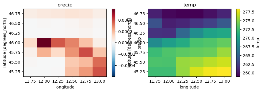
The last RasterDataset file we will add is the era5.nc which consists of climate variables stored in a netcdf file. Let’s open this file with xarray.
[12]:
ds = xr.open_dataset(os.path.join(root, "era5.nc"))
pprint(ds)
<xarray.Dataset> Size: 17kB
Dimensions:      (time: 14, latitude: 7, longitude: 6)
Coordinates:
  * time         (time) datetime64[ns] 112B 2010-02-01 2010-02-02 ... 2010-02-14
  * latitude     (latitude) float32 28B 46.75 46.5 46.25 46.0 45.75 45.5 45.25
  * longitude    (longitude) float32 24B 11.75 12.0 12.25 12.5 12.75 13.0
    spatial_ref  int32 4B ...
Data variables:
    precip       (time, latitude, longitude) float32 2kB ...
    temp         (time, latitude, longitude) float32 2kB ...
    press_msl    (time, latitude, longitude) float32 2kB ...
    kin          (time, latitude, longitude) float32 2kB ...
    kout         (time, latitude, longitude) float32 2kB ...
    temp_min     (time, latitude, longitude) float32 2kB ...
    temp_max     (time, latitude, longitude) float32 2kB ...
Attributes:
    category:        meteo
    history:         Extracted from Copernicus Climate Data Store; resampled ...
    paper_doi:       10.1002/qj.3803
    paper_ref:       Hersbach et al. (2019)
    source_license:  https://cds.climate.copernicus.eu/cdsapp/#!/terms/licenc...
    source_url:      https://doi.org/10.24381/cds.bd0915c6
    source_version:  ERA5 daily data on pressure levels
[13]:
# Select first timestep
ds1 = ds.sel(time=ds.time[0])
ds1
# Plot
fig, axes = plt.subplots(nrows=1, ncols=2, figsize=(10, 3))
ds1["precip"].plot(ax=axes[0])
axes[0].set_title("precip")
ds1["temp"].plot(ax=axes[1])
axes[1].set_title("temp")
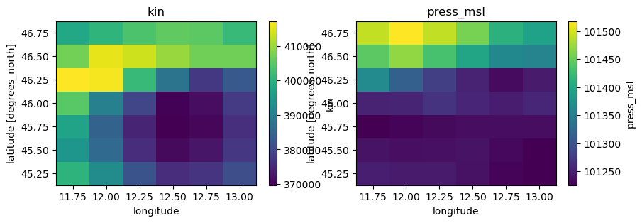
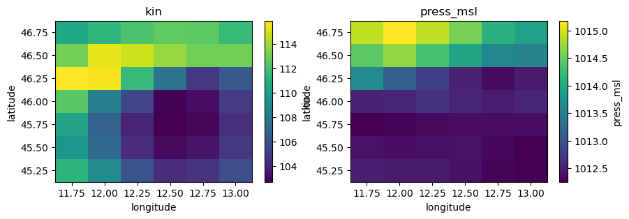
fig, axes = plt.subplots(nrows=1, ncols=2, figsize=(10, 3))
ds1["kin"].plot(ax=axes[0])
axes[0].set_title("kin")
ds1["press_msl"].plot(ax=axes[1])
axes[1].set_title("press_msl")
[13]:
Text(0.5, 1.0, 'press_msl')
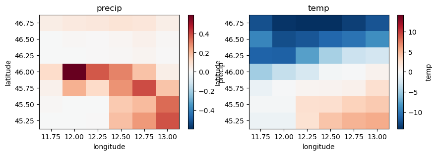
Checking the data conventions we see that all variables already have the right names but the units should be changed:
precip from m to mm
temp, temp_min, temp_max from K to C
kin, kout from J.m-2 to W.m-2
press_msl from Pa to hPa
Let’s change the units using unit_mult and unit_add:
[14]:
yml_str = f"""
meta:
  roots:
  - {root}

era5:
  metadata:
    crs: 4326
  data_type: RasterDataset
  driver:
    name: raster_xarray
  data_adapter:
    unit_add:
      temp: -273.15
      temp_max: -273.15
      temp_min: -273.15
      time: 86400
    unit_mult:
      kin: 0.000277778
      kout: 0.000277778
      precip: 1000
      press_msl: 0.01

  uri: era5.nc

"""
# overwrite data catalog
data_lib = "tmpdir/era5.yml"
with open(data_lib, mode="w") as f:
    f.write(yml_str)
And now open our dataset and check the units have been converted.
[15]:
data_catalog.from_yml(data_lib)  # add a yaml file to the data catalog
print(data_catalog.sources.keys())
ds = data_catalog.get_rasterdataset("era5")
ds
2026-07-02 09:56:03,604 - hydromt.data_catalog.data_catalog - data_catalog - INFO - Parsing data catalog from tmpdir/era5.yml
dict_keys(['vito', 'merit_hydro', 'era5'])
2026-07-02 09:56:03,607 - hydromt.data_catalog.sources.data_source - data_source - INFO - Reading era5 RasterDataset data from /home/runner/.hydromt/artifact_data/v1.0.0/era5.nc
[15]:
<xarray.Dataset> Size: 17kB
Dimensions:      (time: 14, latitude: 7, longitude: 6)
Coordinates:
  * time         (time) datetime64[ns] 112B 2010-02-02 2010-02-03 ... 2010-02-15
  * latitude     (latitude) float32 28B 46.75 46.5 46.25 46.0 45.75 45.5 45.25
  * longitude    (longitude) float32 24B 11.75 12.0 12.25 12.5 12.75 13.0
    spatial_ref  int32 4B ...
Data variables:
    precip       (time, latitude, longitude) float32 2kB dask.array<chunksize=(14, 7, 6), meta=np.ndarray>
    temp         (time, latitude, longitude) float32 2kB dask.array<chunksize=(14, 7, 6), meta=np.ndarray>
    press_msl    (time, latitude, longitude) float32 2kB dask.array<chunksize=(14, 7, 6), meta=np.ndarray>
    kin          (time, latitude, longitude) float32 2kB dask.array<chunksize=(14, 7, 6), meta=np.ndarray>
    kout         (time, latitude, longitude) float32 2kB dask.array<chunksize=(14, 7, 6), meta=np.ndarray>
    temp_min     (time, latitude, longitude) float32 2kB dask.array<chunksize=(14, 7, 6), meta=np.ndarray>
    temp_max     (time, latitude, longitude) float32 2kB dask.array<chunksize=(14, 7, 6), meta=np.ndarray>
Attributes:
    category:        meteo
    history:         Extracted from Copernicus Climate Data Store; resampled ...
    paper_doi:       10.1002/qj.3803
    paper_ref:       Hersbach et al. (2019)
    source_license:  https://cds.climate.copernicus.eu/cdsapp/#!/terms/licenc...
    source_url:      https://doi.org/10.24381/cds.bd0915c6
    source_version:  ERA5 daily data on pressure levels
crs: 4326[16]:
# Select first timestep
ds1 = ds.sel(time=ds.time[0])
ds1
# Plot
fig, axes = plt.subplots(nrows=1, ncols=2, figsize=(10, 3))
ds1["precip"].plot(ax=axes[0])
axes[0].set_title("precip")
ds1["temp"].plot(ax=axes[1])
axes[1].set_title("temp")
fig, axes = plt.subplots(nrows=1, ncols=2, figsize=(10, 3))
ds1["kin"].plot(ax=axes[0])
axes[0].set_title("kin")
ds1["press_msl"].plot(ax=axes[1])
axes[1].set_title("press_msl")
[16]:
Text(0.5, 1.0, 'press_msl')
GeoDataFrame from a vector file#
Now we will see how to add vector data to the data catalogue based on rivers_lin2019_v1.gpkg. Vector files can be open in Python with geopandas (or you can use QGIS) to inspect the data.
[17]:
gdf = gpd.read_file(os.path.join(root, "rivers_lin2019_v1.gpkg"))
pprint(gdf.head())
print(f"Variables: {gdf.columns}")
print(f"CRS: {gdf.crs}")
gdf.plot()
      COMID  order         area       Sin       Slp       Elev             K  \
0  21002594    4.0  1788.131052  1.527056  0.000451  10.648936  3.020000e-11
1  21002602    4.0  1642.386086  1.733917  0.000225  15.861538  3.020000e-11
2  21002675    4.0  2041.630090  1.212651  0.000071   0.975904  3.020000e-11
3  21002937    2.0   258.144582  1.226202  0.000056   1.922830  3.020000e-11
4  21002680    4.0  1983.584528  1.225684  0.000076   1.892537  3.020000e-11

     P        AI       LAI  ...        SLT        Urb       WTD        HW  \
0  0.0  0.795613  1.204846  ...  40.403226  46.983871  1.087777  2.501222
1  0.0  0.828527  1.327503  ...  42.454545  18.181818  4.564060  1.769275
2  0.0  0.662288  0.295892  ...  44.437500  11.250000  0.352534  1.354830
3  0.0  0.726821  1.181066  ...  43.711538  15.634615  1.570532  1.671508
4  0.0  0.719180  1.146002  ...  42.900000  18.900000  0.342745  1.487189

   DOR      QMEAN   qbankfull      rivwth   width_DHG  \
0  0.0  37.047185  190.390803  100.322630   99.347165
1  0.0  35.520306  204.668065  104.193306  103.004818
2  0.0  42.076385  175.181351  125.604490   95.296386
3  0.0   2.426403   23.421744  134.663120   34.845132
4  0.0  41.435879  208.770128  135.457180  104.031935

                                            geometry
0  LINESTRING (11.93917 45.32833, 11.94 45.32917,...
1  LINESTRING (11.83 45.38917, 11.82917 45.38833,...
2  LINESTRING (12.21333 45.19333, 12.2125 45.1941...
3  LINESTRING (12.11 45.23417, 12.10917 45.23417,...
4  LINESTRING (12.1 45.27583, 12.1 45.27667, 12.1...

[5 rows x 22 columns]
Variables: Index(['COMID', 'order', 'area', 'Sin', 'Slp', 'Elev', 'K', 'P', 'AI', 'LAI',
       'SND', 'CLY', 'SLT', 'Urb', 'WTD', 'HW', 'DOR', 'QMEAN', 'qbankfull',
       'rivwth', 'width_DHG', 'geometry'],
      dtype='object')
CRS: EPSG:4326
[17]:
<Axes: >
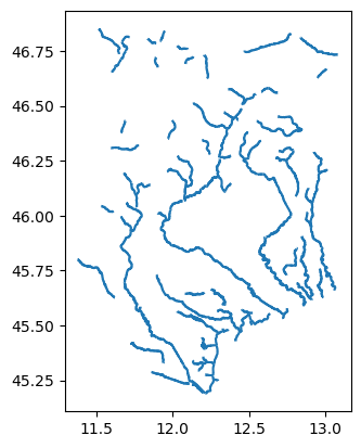
This data source contains rivers line including attributes that can be usefull to setup models such as river width, average discharge or bankfull discharge. Here it’s not needed but feel free to try out some renaming or unit conversion. The minimal data catalog input would be:
[18]:
yml_str = f"""
meta:
  roots:
    - {root}

rivers_lin:
  data_type: GeoDataFrame
  driver:
    name: pyogrio
  uri: rivers_lin2019_v1.gpkg
"""
# overwrite data catalog
data_lib = "tmpdir/rivers.yml"
with open(data_lib, mode="w") as f:
    f.write(yml_str)
[19]:
data_catalog.from_yml(data_lib)  # add a yaml file to the data catalog
print(data_catalog.sources.keys())
gdf = data_catalog.get_geodataframe("rivers_lin")
2026-07-02 09:56:04,278 - hydromt.data_catalog.data_catalog - data_catalog - INFO - Parsing data catalog from tmpdir/rivers.yml
dict_keys(['vito', 'merit_hydro', 'era5', 'rivers_lin'])
2026-07-02 09:56:04,280 - hydromt.data_catalog.sources.data_source - data_source - INFO - Reading rivers_lin GeoDataFrame data from /home/runner/.hydromt/artifact_data/v1.0.0/rivers_lin2019_v1.gpkg
GeoDataset from a netcdf file#
Now we will see how to add geodataset data to the data catalogue based on gtsmv3_eu_era5.nc. This geodataset file contains ocean water level timeseries at specific stations locations in netdcf format and can be opened in Python with xarray. In HydroMT we use a specific wrapper around xarray called GeoDataset to mark that this file contains geospatial timeseries, in this case point timeseries. But for now we can inspect it with xarray.
To learn more about GeoDataset type you can check the reading geodataset example.
[20]:
ds = xr.open_dataset(os.path.join(root, "gtsmv3_eu_era5.nc"))
ds
[20]:
<xarray.Dataset> Size: 323kB
Dimensions:      (time: 2016, stations: 19)
Coordinates:
  * time         (time) datetime64[ns] 16kB 2010-02-01 ... 2010-02-14T23:50:00
  * stations     (stations) int32 76B 13670 2798 2799 13775 ... 2791 2790 2789
    lon          (stations) float64 152B ...
    lat          (stations) float64 152B ...
    spatial_ref  int32 4B ...
Data variables:
waterlevel (time, stations) float64 306kB ...This is quite a classic file, so the data catalog entry is quite straightforward:
[21]:
yml_str = f"""
meta:
  roots:
    - {root}

gtsm:
  data_type: GeoDataset
  driver:
    name: geodataset_xarray
  metadata:
    crs: 4326
    category: ocean
    source_version: GTSM v3.0
  uri: gtsmv3_eu_era5.nc
"""
# overwrite data catalog
data_lib = "tmpdir/gtsm.yml"
with open(data_lib, mode="w") as f:
    f.write(yml_str)
[22]:
data_catalog.from_yml(data_lib)  # add a yaml file to the data catalog
print(data_catalog.sources.keys())
ds = data_catalog.get_geodataset("gtsm")
ds
2026-07-02 09:56:04,309 - hydromt.data_catalog.data_catalog - data_catalog - INFO - Parsing data catalog from tmpdir/gtsm.yml
dict_keys(['vito', 'merit_hydro', 'era5', 'rivers_lin', 'gtsm'])
2026-07-02 09:56:04,312 - hydromt.data_catalog.sources.data_source - data_source - INFO - Reading gtsm GeoDataset data from /home/runner/.hydromt/artifact_data/v1.0.0/gtsmv3_eu_era5.nc
[22]:
<xarray.DataArray 'waterlevel' (time: 2016, stations: 19)> Size: 306kB
dask.array<open_dataset-waterlevel, shape=(2016, 19), dtype=float64, chunksize=(2016, 19), chunktype=numpy.ndarray>
Coordinates:
  * time         (time) datetime64[ns] 16kB 2010-02-01 ... 2010-02-14T23:50:00
  * stations     (stations) int32 76B 13670 2798 2799 13775 ... 2791 2790 2789
    lon          (stations) float64 152B dask.array<chunksize=(19,), meta=np.ndarray>
    lat          (stations) float64 152B dask.array<chunksize=(19,), meta=np.ndarray>
    spatial_ref  int32 4B ...
Attributes:
    long_name:       sea_surface_height_above_mean_sea_level
    units:           m
    CDI_grid_type:   unstructured
    short_name:      waterlevel
    description:     Total water level resulting from the combination of baro...
    category:        ocean
    paper_doi:       10.24381/cds.8c59054f
    paper_ref:       Copernicus Climate Change Service 2019
    source_license:  https://cds.climate.copernicus.eu/cdsapp/#!/terms/licenc...
    source_url:      https://cds.climate.copernicus.eu/cdsapp#!/dataset/10.24...
source_version: GTSM v3.0GeoDataset from vector files#
For geodataset, you can also use the vector driver to combine two files, one for the location and one for the timeseries into one geodataset. We have a custom example available in the data folder of our example notebook using the files stations.csv for the locations and stations_data.csv for the timeseries:
[23]:
# example data folder
root_data = "data"
# let's print some of the file that are there
for item in os.listdir(root_data):
    print(item)
example_csv_data.csv
stations_data.csv
vito_reclass.yml
stations.csv
vito_reclass.csv
tabular_data_catalog.yml
geodataset_catalog.yml
discharge.nc
mesh_model
For this driver to work, the format of the timeseries table is quite strict (see docs). Let’s inspect the two files using pandas in python:
[24]:
df_locs = pd.read_csv("data/stations.csv")
pprint(df_locs)
   stations         x         y
0      1001  12.50244  45.25635
1      1002  12.75879  45.24902
[25]:
df_data = pd.read_csv("data/stations_data.csv")
pprint(df_data)
            time      1001      1002
0     2016-01-01  0.590860  0.591380
1     2016-01-02  0.565552  0.571342
2     2016-01-03  0.538679  0.549770
3     2016-01-04  0.511894  0.526932
4     2016-01-05  0.483989  0.502907
...          ...       ...       ...
2011  2021-07-04  0.271673  0.287093
2012  2021-07-05  0.249286  0.265656
2013  2021-07-06  0.224985  0.243299
2014  2021-07-07  0.199994  0.220004
2015  2021-07-08  0.174702  0.196587

[2016 rows x 3 columns]
And see how the data catalog would look like:
[26]:
yml_str = f"""
meta:
  roots:
    - {os.path.join(os.getcwd(), "data")}

waterlevel_csv:
  metadata:
    crs: 4326
  data_type: GeoDataset
  driver:
    name: geodataset_vector
    options:
      data_path: stations_data.csv
  uri: stations.csv
  data_adapter:
    rename:
      stations_data: waterlevel

"""
# overwrite data catalog
data_lib = "tmpdir/waterlevel.yml"
with open(data_lib, mode="w") as f:
    f.write(yml_str)
[27]:
data_catalog.from_yml(data_lib)  # add a yaml file to the data catalog
print(data_catalog.sources.keys())
ds = data_catalog.get_geodataset("waterlevel_csv")
ds
2026-07-02 09:56:04,365 - hydromt.data_catalog.data_catalog - data_catalog - INFO - Parsing data catalog from tmpdir/waterlevel.yml
dict_keys(['vito', 'merit_hydro', 'era5', 'rivers_lin', 'gtsm', 'waterlevel_csv'])
2026-07-02 09:56:04,367 - hydromt.data_catalog.sources.data_source - data_source - INFO - Reading waterlevel_csv GeoDataset data from /home/runner/work/hydromt/hydromt/docs/_examples/data/stations.csv
[27]:
<xarray.DataArray 'waterlevel' (stations: 2, time: 2016)> Size: 32kB
dask.array<xarray-stations_data, shape=(2, 2016), dtype=float64, chunksize=(2, 2016), chunktype=numpy.ndarray>
Coordinates:
  * stations     (stations) int64 16B 1001 1002
    geometry     (stations) object 16B dask.array<chunksize=(2,), meta=np.ndarray>
  * time         (time) datetime64[ns] 16kB 2016-01-01 2016-01-02 ... 2021-07-08
    spatial_ref  int64 8B 0