Tip

For an interactive online version click here:

Connect Wflow to a 1D model

If you have a Wflow model, one of the applications is that you would like to connect it to a another model such as a 1D hydraulic model like Delft3D or HEC-RAS or a 1D water allocation model like RIBASIM where wflow would give them both river discharge at the boundaries of these models and the runoff generated within the 1D model domain.

HydroMT-Wflow uses a new function setup_1dmodel_connection to try and help you out with these steps. What it does is:

• Add gauges at the 1D model upstream boundaries to exchange river discharge.

• Derive the sub-basins draining into the 1D model river to exchange the amount of water that enters the river (river inwater).

• Optionally, while deriving the sub-basins, large sub-basins can be taken out as tributaries and river discharge is exchanged instead.

Through this notebook we will see some examples of how to use this new function.

Import packages

In this notebook, we will update out Wflow model using python rather than the update command line and do some plotting to visualize the outputs of the function.

from hydromt_wflow import WflowModel
import geopandas as gpd
import numpy as np
from shapely.geometry import box, Point

# Plotting
import matplotlib.pyplot as plt
import cartopy.crs as ccrs

proj = ccrs.PlateCarree()  # plot projection

Connecting to a 1D model

To connect Wflow to a 1D model, we will use the setup_1dmodel_connection.

It uses a 1D river geometry file and there are two methods to connect the models:

• subbasin_area: creates subcatchments linked to the 1d river based on an area threshold (area_max) for the subbasin size. With this method, if a tributary is larger than the area_max, it will be connected to the 1d river directly.

• nodes: subcatchments are derived based on the 1driver nodes (used as gauges locations). With this method, large tributaries can also be derived separately using the add_tributaries option and adding a area_max threshold for the tributaries.

So let’s first load our wflow model and the river file of the 1D model we would like to connect to:

# Load the wflow model of Piave
mod = WflowModel(root="wflow_piave_subbasin", mode="r")

# Open the river of the 1D model
rivers1d = gpd.read_file("data/rivers.geojson")

# And plot the model and the river
# Plot
# we assume the model maps are in the geographic CRS EPSG:4326
proj = ccrs.PlateCarree()
# adjust zoomlevel and figure size to your basis size & aspect
zoom_level = 10
figsize = (10, 8)
shaded = False

# initialize image with geoaxes
fig = plt.figure(figsize=figsize)
ax = fig.add_subplot(projection=proj)
bbox = mod.grid.raster.box.to_crs(3857).buffer(5e3)
extent = np.array(bbox.to_crs(mod.grid.raster.crs).total_bounds)[[0, 2, 1, 3]]
ax.set_extent(extent, crs=proj)

# Wflow
# plot rivers with increasing width with stream order
mod.rivers.plot(ax=ax, lw=mod.rivers["strord"] / 2, color="blue", zorder=3, label=" wflow river")
# plot the basin boundary
mod.basins.boundary.plot(ax=ax, color="k", linewidth=0.5)

# 1D river
rivers1d.to_crs(mod.crs).plot(ax=ax, color="red", linewidth=2, zorder=4, label="1D river")

ax.xaxis.set_visible(True)
ax.yaxis.set_visible(True)
ax.set_ylabel(f"latitude [degree north]")
ax.set_xlabel(f"longitude [degree east]")
_ = ax.set_title(f"Wflow model and 1D river network of Piave subbasin")
legend = ax.legend(
    handles=[*ax.get_legend_handles_labels()[0]],
    title="Legend",
    loc="lower right",
    frameon=True,
    framealpha=0.7,
    edgecolor="k",
    facecolor="white",
)

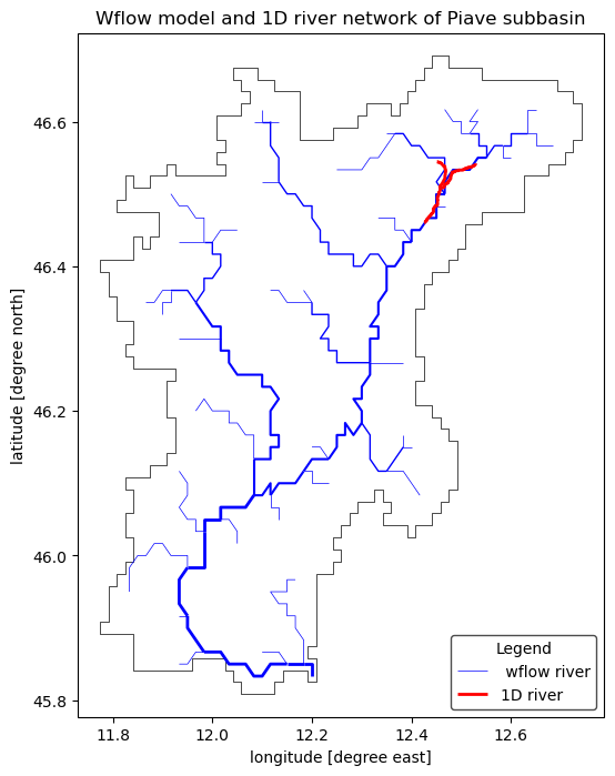
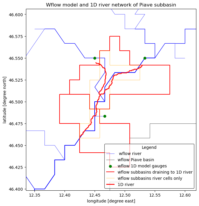
Subbasin area connection method and tributaries

We see that our 1D model is located in the Northern part of our Wflow model.

Let’s connect the two using the subbasin_area method and including tributaries for subbasins that are larger than 30 km2.

# Run the setup_1d_model_connection function
mod.setup_1dmodel_connection(
    river1d_fn=rivers1d,
    connection_method="subbasin_area",
    area_max=30.0,
    add_tributaries=True,
    include_river_boundaries=True,
    mapname="1dmodel",
    update_toml=True,
    toml_output="netcdf",
)

We can see than in that case the toml was already updated to save the relevant outputs for our new gauges and subcatch:

mod.config["netcdf"]

{'path': 'output_scalar.nc',
 'variable': [{'name': 'Q',
   'map': 'gauges_1dmodel',
   'parameter': 'lateral.river.q_av'},
  {'name': 'Qlat',
   'map': 'subcatch_riv_1dmodel',
   'parameter': 'lateral.river.inwater',
   'reducer': 'sum'}]}

And let’s visualize our results:

# And plot the model and the river
# Plot
# we assume the model maps are in the geographic CRS EPSG:4326
proj = ccrs.PlateCarree()
# adjust zoomlevel and figure size to your basis size & aspect
zoom_level = 10
figsize = (10, 8)
shaded = False

# initialize image with geoaxes
fig = plt.figure(figsize=figsize)
ax = fig.add_subplot(projection=proj)
bbox = gpd.GeoDataFrame(geometry=[box(*rivers1d.total_bounds)], crs=rivers1d.crs)
bbox = bbox.buffer(10e3)
extent = np.array(bbox.to_crs(mod.grid.raster.crs).total_bounds)[[0, 2, 1, 3]]
ax.set_extent(extent, crs=proj)

# Wflow
# plot rivers with increasing width with stream order
mod.rivers.plot(ax=ax, lw=mod.rivers["strord"] / 2, color="blue", zorder=3, label=" wflow river")
# plot the basin boundary
mod.basins.boundary.plot(ax=ax, color="k", linewidth=0.5, label="wflow Piave basin")
# Add the boundry gauges and tributary gauges
if "gauges_1dmodel" in mod.geoms:
    mod.geoms["gauges_1dmodel"].plot(ax=ax, color="green", zorder=4, label="wflow 1D model gauges")
# Add the full subbasins and river only
mod.geoms["subcatch_1dmodel"].boundary.plot(ax=ax, color='red', zorder=4, label="wflow subbasins draining to 1D river")
mod.geoms["subcatch_riv_1dmodel"].boundary.plot(ax=ax, color="orange", linewidth=0.5, zorder=4, label="wflow subbasins river cells only")

# 1D river
rivers1d.to_crs(mod.crs).plot(ax=ax, color="red", linewidth=2, zorder=5, label="1D river")

ax.xaxis.set_visible(True)
ax.yaxis.set_visible(True)
ax.set_ylabel(f"latitude [degree north]")
ax.set_xlabel(f"longitude [degree east]")
_ = ax.set_title(f"Wflow model and 1D river network of Piave subbasin")
legend = ax.legend(
    handles=[*ax.get_legend_handles_labels()[0]],
    title="Legend",
    loc="lower right",
    frameon=True,
    framealpha=0.7,
    edgecolor="k",
    facecolor="white",
)

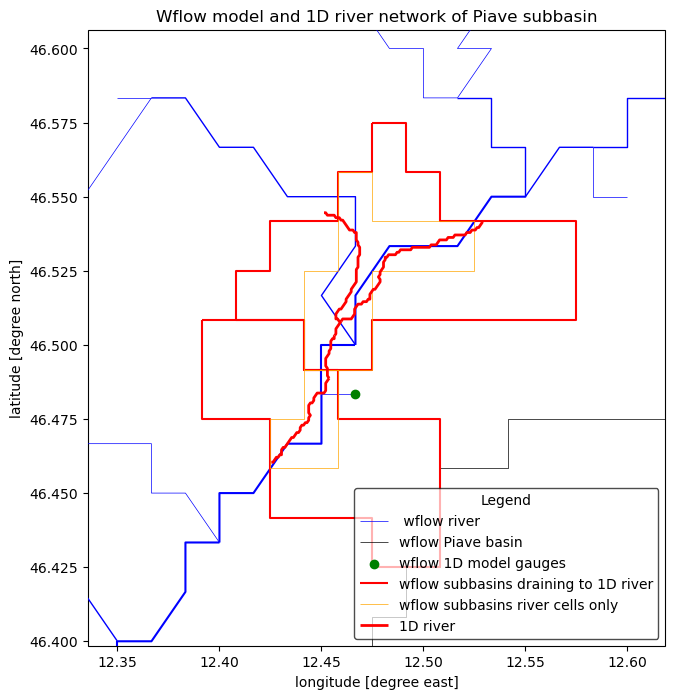
Let’s try the same if we do not include river boundaries:

# Run the setup_1d_model_connection function
mod1 = WflowModel(root="wflow_piave_subbasin", mode="r")
mod1.setup_1dmodel_connection(
    river1d_fn=rivers1d,
    connection_method="subbasin_area",
    area_max=30.0,
    add_tributaries=True,
    include_river_boundaries=False,
    mapname="1dmodel",
    update_toml=True,
    toml_output="netcdf",
)

# And plot the model and the river
# Plot
# we assume the model maps are in the geographic CRS EPSG:4326
proj = ccrs.PlateCarree()
# adjust zoomlevel and figure size to your basis size & aspect
zoom_level = 10
figsize = (10, 8)
shaded = False

# initialize image with geoaxes
fig = plt.figure(figsize=figsize)
ax = fig.add_subplot(projection=proj)
bbox = gpd.GeoDataFrame(geometry=[box(*rivers1d.total_bounds)], crs=rivers1d.crs)
bbox = bbox.buffer(10e3)
extent = np.array(bbox.to_crs(mod.grid.raster.crs).total_bounds)[[0, 2, 1, 3]]
ax.set_extent(extent, crs=proj)

# Wflow
# plot rivers with increasing width with stream order
mod1.rivers.plot(ax=ax, lw=mod1.rivers["strord"] / 2, color="blue", zorder=3, label=" wflow river")
# plot the basin boundary
mod1.basins.boundary.plot(ax=ax, color="k", linewidth=0.5, label="wflow Piave basin")
# Add the boundry gauges and tributary gauges
mod1.geoms["gauges_1dmodel"].plot(ax=ax, color="green", zorder=4, label="wflow 1D model gauges")
# Add the full subbasins and river only
mod1.geoms["subcatch_1dmodel"].boundary.plot(ax=ax, color='red', zorder=4, label="wflow subbasins draining to 1D river")
mod1.geoms["subcatch_riv_1dmodel"].boundary.plot(ax=ax, color="orange", linewidth=0.5, zorder=4, label="wflow subbasins river cells only")

# 1D river
rivers1d.to_crs(mod1.crs).plot(ax=ax, color="red", linewidth=2, zorder=5, label="1D river")

ax.xaxis.set_visible(True)
ax.yaxis.set_visible(True)
ax.set_ylabel(f"latitude [degree north]")
ax.set_xlabel(f"longitude [degree east]")
_ = ax.set_title(f"Wflow model and 1D river network of Piave subbasin")
legend = ax.legend(
    handles=[*ax.get_legend_handles_labels()[0]],
    title="Legend",
    loc="lower right",
    frameon=True,
    framealpha=0.7,
    edgecolor="k",
    facecolor="white",
)

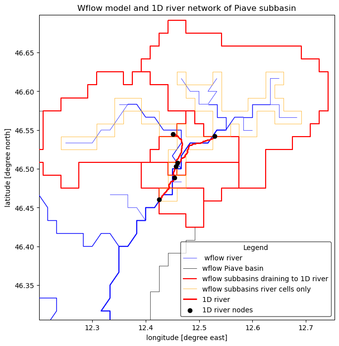
Nodes connection method

This connection is different as we create subbasins only for all nodes of the 1D river file. Let’s see the difference:

# Run the setup_1d_model_connection function
mod1 = WflowModel(root="wflow_piave_subbasin", mode="r")
mod1.setup_1dmodel_connection(
    river1d_fn=rivers1d,
    connection_method="nodes",
    area_max=30.0,
    add_tributaries=False,
    include_river_boundaries=False,
    mapname="1dmodel",
    update_toml=False,
)

# And plot the model and the river
# Plot
# we assume the model maps are in the geographic CRS EPSG:4326
proj = ccrs.PlateCarree()
# adjust zoomlevel and figure size to your basis size & aspect
zoom_level = 10
figsize = (10, 8)
shaded = False

# initialize image with geoaxes
fig = plt.figure(figsize=figsize)
ax = fig.add_subplot(projection=proj)
bbox = gpd.GeoDataFrame(geometry=[box(*rivers1d.total_bounds)], crs=rivers1d.crs)
bbox = bbox.buffer(25e3)
extent = np.array(bbox.to_crs(mod.grid.raster.crs).total_bounds)[[0, 2, 1, 3]]
ax.set_extent(extent, crs=proj)

# Wflow
# plot rivers with increasing width with stream order
mod1.rivers.plot(ax=ax, lw=mod1.rivers["strord"] / 2, color="blue", zorder=3, label=" wflow river")
# plot the basin boundary
mod1.basins.boundary.plot(ax=ax, color="k", linewidth=0.5, label="wflow Piave basin")
# Add the full subbasins and river only
mod1.geoms["subcatch_1dmodel"].boundary.plot(ax=ax, color='red', zorder=4, label="wflow subbasins draining to 1D river")
mod1.geoms["subcatch_riv_1dmodel"].boundary.plot(ax=ax, color="orange", linewidth=0.5, zorder=4, label="wflow subbasins river cells only")

# 1D river
rivers1d.to_crs(mod1.crs).plot(ax=ax, color="red", linewidth=2, zorder=5, label="1D river")
# Plot the rivers1d nodes
nodes = []
for bi, branch in rivers1d.iterrows():
    nodes.append([Point(branch.geometry.coords[0]), bi])  # start
    nodes.append([Point(branch.geometry.coords[-1]), bi])  # end
gdf_nodes = gpd.GeoDataFrame(
    nodes, columns=["geometry", "river_id"], crs=rivers1d.crs
)
# Drop duplicates geometry
gdf_nodes = gdf_nodes[~gdf_nodes.geometry.duplicated(keep="first")]
gdf_nodes.to_crs(mod1.crs).plot(ax=ax, color="black", zorder=6, label="1D river nodes")

ax.xaxis.set_visible(True)
ax.yaxis.set_visible(True)
ax.set_ylabel(f"latitude [degree north]")
ax.set_xlabel(f"longitude [degree east]")
_ = ax.set_title(f"Wflow model and 1D river network of Piave subbasin")
legend = ax.legend(
    handles=[*ax.get_legend_handles_labels()[0]],
    title="Legend",
    loc="lower right",
    frameon=True,
    framealpha=0.7,
    edgecolor="k",
    facecolor="white",
)