RA2CE feature: Equity analysis#
This notebook is aimed at users with background knowledge of network criticality analysis.
In this notebook, we perform criticality analysis using three different distributive principles: utilitarian, egalitarian, and prioritarian. For more background on these principles and their application to transport network criticality analysis, please read: https://www.sciencedirect.com/science/article/pii/S0965856420308077
The purpose of the equity analysis performed in this notebook is to provide insight into how different distributive principles can result in different prioritisations of the network. While we usually prioritise network interventions based on the number of people using a road, equity principles also allow us to take into account the role of the network for underprivileged communities. Depending on the equity principle applied, your network prioritisation may change, which can affect decision-making.
The RA2CE analysis is set up generically: the user can define the equity weights themselves. These can be, for example, Gini coefficients or social vulnerability scores. The user-defined equity weights feed into the prioritarian principle.
The three applied principles are explained below:

For new users#
If you have not checked out the previous RA2CE examples and you want to run your own RA2CE analysis, we advise you to first familiarize yourself with those notebooks. In this current notebook we will not provide extensive explanations as to how to run RA2CE and create the correct setups. We will assume the user has this knowledge already.
This equity notebook is an extension of the accessibility analysis (Origin-Destination).
Imports#
Import all required packages and set the path to your RA2CE project folder.
[17]:
from pathlib import Path

import folium
import geopandas as gpd
import matplotlib.pyplot as plt
import pandas as pd

from ra2ce.analysis.analysis_config_data.analysis_config_data import AnalysisConfigData, AnalysisSectionLosses
from ra2ce.analysis.analysis_config_data.enums.analysis_losses_enum import AnalysisLossesEnum
from ra2ce.analysis.analysis_config_data.enums.weighing_enum import WeighingEnum
from ra2ce.network.network_config_data.enums.network_type_enum import NetworkTypeEnum
from ra2ce.network.network_config_data.enums.road_type_enum import RoadTypeEnum
from ra2ce.network.network_config_data.enums.source_enum import SourceEnum
from ra2ce.network.network_config_data.network_config_data import (
    NetworkConfigData,
    NetworkSection,
    OriginsDestinationsSection,
)
from ra2ce.ra2ce_handler import Ra2ceHandler

# Specify the path to your RA2CE project folder and input data
root_dir = Path("data", "equity_analysis")
network_path = root_dir / "static" / "network"
Inspect data and get familiar with the use-case#
Below we inspect the input data for the Pontianak, Indonesia use case. Before running sections 1 and 2, make sure your own data is prepared and stored in the correct folder (see the note at the end of this section).
1. Using equity weights to delineate more vulnerable areas#
For the equity analysis, the user assigns equity weights that are used in the criticality calculation. In this example we use a region weights file (region_weight.csv) containing weights for specific administrative areas in Pontianak, Indonesia. A shapefile delineating those regions is also required. We inspect both files here and identify which areas are considered more vulnerable according to the user-specified equity weights.
[18]:
path_region_weights = network_path / "region_weight.csv"
path_regions = network_path / "region.shp"

region_weights = pd.read_csv(path_region_weights, sep=";")
regions = gpd.read_file(path_regions)

# Merge the shapefile and the weights CSV file
region_weights_plot = pd.merge(regions, region_weights, left_on="DESA", right_on="region")
The map below shows vulnerability weights per region: darker red indicates a higher weight (more vulnerable area).
[32]:
region_weights_plot.explore(column="weight", cmap="Reds", tiles="CartoDB positron")
[32]:
2. Inspect origins, destinations and the road network#
Load the origin and destination point datasets for this analysis. Origins represent populated areas (WorldPop grid cells); destinations represent health facilities.
[20]:
path_origins = network_path / "origins_points.shp"
path_destinations = network_path / "osm_health_point.shp"
origins = gpd.read_file(path_origins)
destinations = gpd.read_file(path_destinations)
The map below shows origin points in blue (population centroids) and health facility destinations in red. Use the layer control to toggle each layer.
[ ]:
m = origins.explore(color="blue", tiles="CartoDB positron", name="WorldPop origins")
m = destinations.explore(m=m, color="red", name="Health destinations")
folium.LayerControl().add_to(m)
m
Before running your own analysis: data checklist#
If you want to run this notebook with your own data, check the following before proceeding:
Review the origins/destinations example notebook to understand how to prepare those files.
Ensure your
region.shpandregion_weight.csvfiles are saved indata/equity_analysis/static/network/.Confirm the column name used for region identifiers matches between the shapefile and the CSV (in this example:
DESAandregionrespectively).
Run the RA2CE analysis#
Configure the network, origin-destination settings, and analysis parameters, then run the handler. The results will be written to data/equity_analysis/output/.
[ ]:
network_section = NetworkSection(
    directed=False,
    source=SourceEnum.OSM_DOWNLOAD,
    polygon=network_path / "Pontianak_4326_buffer_0_025deg.geojson",
    network_type=NetworkTypeEnum.DRIVE,
    road_types=[
        RoadTypeEnum.MOTORWAY,
        RoadTypeEnum.MOTORWAY_LINK,
        RoadTypeEnum.PRIMARY,
        RoadTypeEnum.PRIMARY_LINK,
        RoadTypeEnum.SECONDARY,
        RoadTypeEnum.SECONDARY_LINK,
        RoadTypeEnum.TERTIARY,
        RoadTypeEnum.TERTIARY_LINK,
    ],
    save_gpkg=True,
    reuse_network_output=True,
)

origin_destination_section = OriginsDestinationsSection(
    origins=network_path / "origins_points.shp",
    destinations=network_path / "osm_health_point.shp",
    origin_count="values",
    category="category",
    region=network_path / "region.shp",
    region_var="DESA",
)
[23]:
network_config_data = NetworkConfigData(
    root_path=root_dir,
    static_path=root_dir.joinpath('static'),
    network=network_section,
    origins_destinations=origin_destination_section,
)
[24]:
analyse_section = AnalysisSectionLosses(
    name="Optimal Route OD equity",
    analysis=AnalysisLossesEnum.OPTIMAL_ROUTE_ORIGIN_DESTINATION,
    weighing=WeighingEnum.LENGTH,
    calculate_route_without_disruption=True,
    equity_weight='region_weight.csv',
    save_traffic =True,
    save_csv=True,
    save_gpkg=True,
)

analysis_config_data = AnalysisConfigData(
    output_path=root_dir.joinpath("output"),
    static_path=root_dir.joinpath('static'),
    analyses=[analyse_section],
)
Run the analysis. RA2CE will compute optimal routes between all origin–destination pairs and produce three traffic columns: traffic (utilitarian), traffic_egalitarian, and traffic_prioritarian.
[25]:
handler = Ra2ceHandler.from_config(
    network=network_config_data,
    analysis=analysis_config_data
)
handler.configure()
handler.run_analysis()
Finding optimal routes.: 100%|██████████| 540/540 [00:00<00:00, 1611.76it/s]
[25]:
[AnalysisResultWrapper(results_collection=[AnalysisResult(analysis_result=          o_node       d_node origin destination  \
 0    13081248522  13081248617    O_0         D_0
 1    13081248522  13081248618    O_0         D_1
 2    13081248522  13081248619    O_0         D_2
 3    13081248522  13081248620    O_0         D_3
 4    13081248522  13081248621    O_0         D_4
 ..           ...          ...    ...         ...
 205  13081248611  13081248617  O_102         D_0
 206  13081248611  13081248618  O_102         D_1
 207  13081248611  13081248619  O_102         D_2
 208  13081248611  13081248620  O_102         D_3
 209  13081248611  13081248621  O_102         D_4

                                               opt_path    length  \
 0    [13081248522, 13081248525, 10736480779, 130812...  4866.936
 1    [13081248522, 13081248525, 10736480779, 130812...  7642.585
 2    [13081248522, 13081248525, 10736480779, 130812...  6852.543
 3    [13081248522, 13081248525, 10736480779, 130812...  7917.141
 4    [13081248522, 13081248525, 10736480779, 130812...  8099.070
 ..                                                 ...       ...
 205  [13081248611, 586717899, 2530351154, 130812486...  6966.572
 206  [13081248611, 586717899, 2530351154, 130812486...  6590.588
 207  [13081248611, 586717899, 2530351154, 130812486...  5800.546
 208  [13081248611, 586717899, 2530351154, 130812486...  3917.166
 209  [13081248611, 586717899, 2530351154, 130812486...  3734.438

                                              match_ids  \
 0    [295, 295, 364, 364, 303, 301, 301, 299, 299, ...
 1    [295, 295, 364, 364, 303, 301, 301, 299, 299, ...
 2    [295, 295, 364, 364, 303, 301, 301, 299, 299, ...
 3    [295, 295, 364, 364, 303, 301, 301, 299, 299, ...
 4    [295, 295, 364, 364, 303, 301, 301, 299, 299, ...
 ..                                                 ...
 205  [276, 150, 151, 151, 148, 147, 147, 233, 229, ...
 206  [276, 150, 151, 151, 148, 147, 147, 233, 229, ...
 207  [276, 150, 151, 151, 148, 147, 147, 233, 229, ...
 208  [276, 150, 151, 151, 148, 147, 147, 233, 229, ...
 209  [276, 150, 151, 151, 148, 147, 147, 233, 229, ...

                                               geometry
 0    MULTILINESTRING ((109.28661 -0.03797, 109.2869...
 1    MULTILINESTRING ((109.28661 -0.03797, 109.2869...
 2    MULTILINESTRING ((109.28661 -0.03797, 109.2869...
 3    MULTILINESTRING ((109.28661 -0.03797, 109.2869...
 4    MULTILINESTRING ((109.28661 -0.03797, 109.2869...
 ..                                                 ...
 205  MULTILINESTRING ((109.36368 -0.05675, 109.3633...
 206  MULTILINESTRING ((109.36368 -0.05675, 109.3633...
 207  MULTILINESTRING ((109.36368 -0.05675, 109.3633...
 208  MULTILINESTRING ((109.36368 -0.05675, 109.3633...
 209  MULTILINESTRING ((109.36368 -0.05675, 109.3633...

 [210 rows x 8 columns], analysis_config=AnalysisSectionLosses(name='Optimal Route OD equity', save_gpkg=True, save_csv=True, analysis=<AnalysisLossesEnum.OPTIMAL_ROUTE_ORIGIN_DESTINATION: 3>, weighing=<WeighingEnum.LENGTH: 1>, production_loss_per_capita_per_hour=nan, traffic_period=<TrafficPeriodEnum.DAY: 1>, hours_per_traffic_period=0, trip_purposes=[<TripPurposeEnum.NONE: 0>], resilience_curves_file=None, traffic_intensities_file=None, values_of_time_file=None, threshold=0.0, threshold_destinations=nan, equity_weight='region_weight.csv', calculate_route_without_disruption=True, buffer_meters=nan, category_field_name='', save_traffic=True, event_type=<EventTypeEnum.NONE: 0>, risk_calculation_mode=<RiskCalculationModeEnum.NONE: 0>, risk_calculation_year=0), output_path=WindowsPath('data/equity_analysis/output'), _custom_name='')])]
Post-processing results#
The results are saved under output/optimal_route_origin_destination/ as a CSV without geometry. The steps below join those results to the network edges GeoPackage so they can be mapped.
1. Load the traffic analysis output#
[26]:
optimal_route = root_dir/'output'/'optimal_route_origin_destination'
optimal_route_graph = optimal_route / "Optimal_Route_OD_equity_link_traffic.csv"
traffic = pd.read_csv(optimal_route_graph)
df = traffic.copy()
df.head()
[26]:
| u | v | traffic | traffic_egalitarian | traffic_prioritarian | |
|---|---|---|---|---|---|
| 0 | 13081248522 | 13081248525 | 8.144307 | 5.0 | 6.446749 |
| 1 | 13081248525 | 10736480779 | 3585.867208 | 10.0 | 2838.447155 |
| 2 | 10736480779 | 13081248524 | 3585.867208 | 10.0 | 2838.447155 |
| 3 | 13081248524 | 7238291279 | 4814.463765 | 15.0 | 3810.961251 |
| 4 | 7238291279 | 7238291270 | 4814.463765 | 15.0 | 3810.961251 |
2. Load the graph edges (with geometry)#
[ ]:
path_output_graph = root_dir / "static" / "output_graph"
base_graph_edges = path_output_graph / "origins_destinations_graph_edges.gpkg"
gdf = gpd.read_file(base_graph_edges)
gdf.head()
| u | v | key | oneway | name | highway | reversed | length | rfid_c | rfid | ... | bridge | node_A | node_B | edge_fid | lanes | width | junction | access | osmid_original | geometry | |
|---|---|---|---|---|---|---|---|---|---|---|---|---|---|---|---|---|---|---|---|---|---|
| 0 | 559431729 | 1848302290 | 0 | True | Jalan Agus Salim | tertiary | False | 9.178 | 4 | 1 | ... | nan | NaN | NaN | nan | nan | nan | nan | nan | 782412294 | LINESTRING (109.33922 -0.02962, 109.33915 -0.0... |
| 1 | 559431729 | 559431731 | 0 | True | Jalan Gajah Mada | tertiary | False | 127.113 | [1313, 3, 7133, 2779] | 2 | ... | nan | NaN | NaN | nan | nan | nan | nan | nan | 43996468 | LINESTRING (109.33922 -0.02962, 109.33930 -0.0... |
| 2 | 559431729 | 1977410506 | 0 | True | nan | tertiary | False | 13.663 | 726 | 76 | ... | nan | NaN | NaN | nan | nan | nan | nan | nan | 575398528 | LINESTRING (109.33922 -0.02962, 109.33916 -0.0... |
| 3 | 559431729 | 1977410544 | 0 | True | Jalan Agus Salim | tertiary | False | 73.745 | [7129, 739] | 79 | ... | nan | NaN | NaN | nan | nan | nan | nan | nan | 43996479 | LINESTRING (109.33976 -0.02924, 109.33934 -0.0... |
| 4 | 559431731 | 5891888009 | 0 | True | Jalan Gajah Mada | tertiary | False | 187.868 | [800, 801, 5, 6664, 4210, 2168, 2169, 4253] | 3 | ... | nan | NaN | NaN | nan | nan | nan | nan | nan | 43996468 | LINESTRING (109.33975 -0.03064, 109.33989 -0.0... |
5 rows × 22 columns
3. Merge traffic values onto the edge geometries#
For each edge (u, v) in the network, we look up the corresponding traffic value from the analysis output. Because the graph is undirected, we also check the reverse edge (v, u) for edges that were stored in the opposite direction.
[ ]:
traffic_cols = ["u", "v", "traffic", "traffic_egalitarian", "traffic_prioritarian"]

# Try forward edges (u→v) first, then reverse (v→u) for undirected graphs
fwd = df[traffic_cols]
rev = df[traffic_cols].rename(columns={"u": "v", "v": "u"})

merged_fwd = gdf[["u", "v"]].merge(fwd, on=["u", "v"], how="left")
merged_rev = gdf[["u", "v"]].merge(rev, on=["u", "v"], how="left")

for var in ["traffic", "traffic_egalitarian", "traffic_prioritarian"]:
    gdf[var] = merged_fwd[var].fillna(merged_rev[var]).fillna(0)
4. Rank edges by traffic under each principle#
Rank 1 = most critical edge. Edges with zero traffic (unreachable or unused) receive the lowest ranks.
[29]:
gdf['traffic_ranked'] = gdf['traffic'].rank(method='min', ascending=False)
gdf['traffic_egalitarian_ranked'] = gdf['traffic_egalitarian'].rank(method='min', ascending=False)
gdf['traffic_prioritarian_ranked'] = gdf['traffic_prioritarian'].rank(method='min', ascending=False)
Visualize results#
The three maps below compare edge criticality rankings under each distributive principle. Darker (hotter) colours indicate a higher rank (rank 1 = most critical). Edges that appear critical under one principle but not another are where the principles diverge most.
[30]:
fig, axs = plt.subplots(1, 3, figsize=(15, 5))

gdf.plot(column="traffic_ranked", cmap="gist_heat", ax=axs[0], legend=True)
axs[0].set_title("Utilitarian principle ranking")
axs[0].axis("off")

gdf.plot(column="traffic_egalitarian_ranked", cmap="gist_heat", ax=axs[1], legend=True)
axs[1].set_title("Egalitarian principle ranking")
axs[1].axis("off")

gdf.plot(column="traffic_prioritarian_ranked", cmap="gist_heat", ax=axs[2], legend=True)
axs[2].set_title("Prioritarian principle ranking")
axs[2].axis("off")

plt.tight_layout()
plt.show()
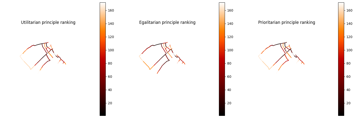
How to read these maps:
Utilitarian: ranks edges by the total number of people using them. The most-used roads rank highest.
Egalitarian: treats every origin–destination pair equally, regardless of population size. A road serving a small but isolated community can rank as highly as one serving a dense area.
Prioritarian: weights travel by the user-supplied equity scores. Roads that connect underprivileged areas receive higher effective demand and therefore rank higher.
Edges that look the same across all three maps are robustly critical regardless of the principle chosen. Edges that shift rank significantly are the ones where the choice of principle matters most for investment decisions.
These results can directly inform network investment prioritisation. If the goal is to serve underprivileged communities, the prioritarian ranking — combined with weights that reflect social vulnerability — will highlight different roads than a purely utilitarian approach. Because the user is free to specify their own equity weights, the analysis can be adapted to any local context or policy objective.
Interactive map: Prioritarian ranking#
The interactive map below shows the full network coloured by prioritarian rank. Zoom in to explore individual edges and compare with the static overview above.
[33]:
tooltip_cols = [
    "name", "highway", "length",
    "traffic_ranked", "traffic_egalitarian_ranked", "traffic_prioritarian_ranked",
]

gdf.explore(
    column="traffic_prioritarian_ranked",
    tiles="CartoDB positron",
    cmap="gist_heat",
    tooltip=tooltip_cols,
)
[33]:
[ ]: