In this example, we’ll work with an unstructured grid. We’ll create a very simple unstructured model of the Netherlands from scratch. We’ll use a digital elevation model (DEM) to set as drain level to simulate overland flow. To this we add constant recharge.

Let’s start with importing the required packages. These are iMOD Python, xarray, and xugrid.

import imod
import xarray as xr
import xugrid as xu

/home/runner/work/iMOD-Documentation/iMOD-Documentation/.pixi/envs/default/lib/python3.14/site-packages/tqdm/auto.py:21: TqdmWarning: IProgress not found. Please update jupyter and ipywidgets. See https://ipywidgets.readthedocs.io/en/stable/user_install.html
  from .autonotebook import tqdm as notebook_tqdm

Load the data

This data is distributed with the xugrid package. You need an internet connection to download the data.


elevation = xu.data.elevation_nl()

elevation

Downloading file 'elevation_nl.nc' from 'https://github.com/deltares/xugrid/raw/main/data/elevation_nl.nc' to '/home/runner/.cache/xugrid'.

<xarray.DataArray 'elevation' (mesh2d_nFaces: 5248)> Size: 21kB
[5248 values with dtype=float32]
Coordinates:
  * mesh2d_nFaces  (mesh2d_nFaces) int64 42kB 0 1 2 3 4 ... 5244 5245 5246 5247
    mesh2d_face_x  (mesh2d_nFaces) float64 42kB ...
    mesh2d_face_y  (mesh2d_nFaces) float64 42kB ...
Attributes:
    unit:     m NAP

Let’s plot the data

elevation.ugrid.plot(vmin=-20, vmax=90, cmap="terrain")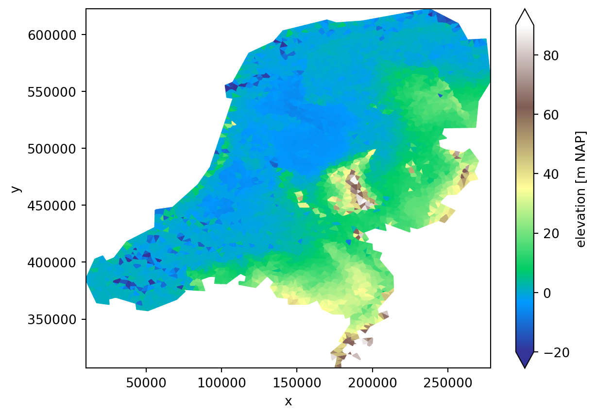

Template grid

It is convenient to create a template grid, which has the right shape, dimensions, and coordinates. This can be used to construct DataArrays for different variables.

We’ll start off with creating a layer DataArray, which is a 1D DataArray, containing all layer information required.

layer = xr.DataArray(data=[1], coords={"layer": [1]}, dims=("layer",))

layer

<xarray.DataArray (layer: 1)> Size: 8B
array([1])
Coordinates:
  * layer    (layer) int64 8B 1

Next, we’ll create a 2D planar template grid. The xarray function .ones_like returns a new object of ones with the same shape and type as a given dataarray or dataset.

template_2d = imod.typing.grid.ones_like(elevation, dtype=int)

template_2d

<xarray.DataArray 'elevation' (mesh2d_nFaces: 5248)> Size: 42kB
array([1, 1, 1, ..., 1, 1, 1], shape=(5248,))
Coordinates:
  * mesh2d_nFaces  (mesh2d_nFaces) int64 42kB 0 1 2 3 4 ... 5244 5245 5246 5247
    mesh2d_face_x  (mesh2d_nFaces) float64 42kB ...
    mesh2d_face_y  (mesh2d_nFaces) float64 42kB ...
Attributes:
    unit:     m NAP

Finally, we’ll create our unstructured template 3D grid.

We’ll multiply our template 2d grid with the layer template to construct the full 3D grid. Pay attention to the dimension order, iMOD Python is very specific about this. We’ll put the dimensions in the right order immediately, to save ourselves headaches later.

# iMOD Python requires the layer dimension first, faces dimension second
template = (template_2d * layer).transpose("layer", "mesh2d_nFaces")
# plot
template.sel(layer=1).ugrid.plot(vmin=0, vmax=2, cmap="viridis")

Drainage

We can now use the template grid to transform the 2D elevation grid to a 3D elevation grid, required for the drainage package.

# Drain info
drainage_lvl = template * elevation  # requires layer dimension
# plot
drainage_lvl.sel(layer=1).ugrid.plot(vmin=-5, vmax=40, cmap="viridis")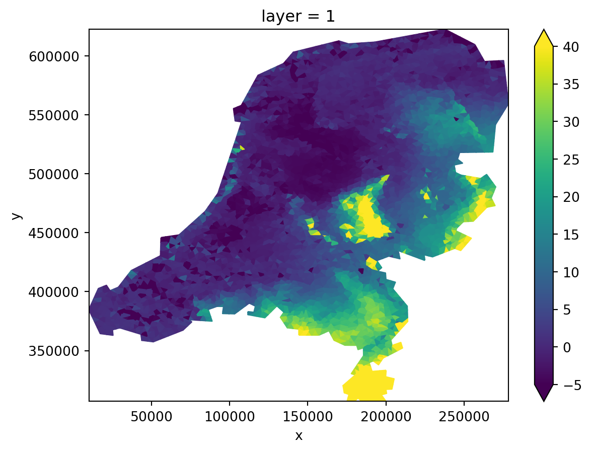

Compute conductance. The function .ugrid.grid.area yields a numpy array with for each unstructured element its area (m2). Multiplied with the unstructured grid with value 1 yiels grid with area.

cell_area = template * template.ugrid.grid.area # [m2]
resistance = 1  # [d]
conductance = cell_area / resistance # [m2/d]
# Plot
conductance.sel(layer=1).ugrid.plot()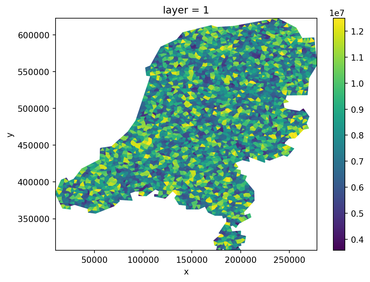

Discretization

Prepare our model discretization. idomain specifies whether a call is active [1], inactive [0], or vertical pass through [-1]. In this case we’ll go for a grid that is active everywhere.


idomain = template.copy()

We’ll also define the bottom of the model. To keep things simple, we’ll subtract 300 from the drainage level, which will also be our top. In this way, we’ll construct a model with thickness 300 everywhere.

bottom = drainage_lvl - 300.0
# Plot
bottom.sel(layer=1).ugrid.plot()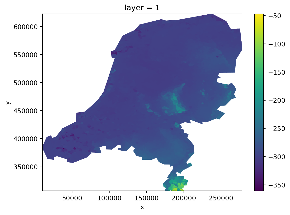

Recharge

Let’s prepare our recharge. Note that Modflow 6 requires consistent length units, so we have to provide recharge in m/d instead of mm/d!

# Define recharge
recharge_rate = template * 0.002
# Plot
recharge_rate.sel(layer=1).ugrid.plot()

Construct simulation

Initialization of the main MODFLOW 6 object. We give it a name.

simulation = imod.mf6.Modflow6Simulation("nl_elevation")

Within a Modflow6Simulation object one or more models can be defined. In this example there is just one ground water flow model.
In the next cells we will assemble our groundwater model in the object “gwf_model”. Further down, we add it to the object “simulation”.

In the next cell we define that option newton is chosen.

gwf_model = imod.mf6.GroundwaterFlowModel(newton=True)

The DIS package with vertices discretization needs input on tops, bottom and idomain.

gwf_model["dis"] = imod.mf6.VerticesDiscretization(
    top=elevation, idomain=idomain, bottom=bottom
)

Assign storage package:

gwf_model["sto"] = imod.mf6.SpecificStorage(
    specific_storage=1e-5, specific_yield=0.01, transient=False, convertible=1
)

Assign initial conditions, we’ll set them equal to drainage level.

gwf_model["ic"] = imod.mf6.InitialConditions(start=drainage_lvl)

The Node Property Flow is most noteworthy where we specify the hydraulic conductivities. For a simple homogeneous, isotropic medium of 10 m/d:

gwf_model["npf"] = imod.mf6.NodePropertyFlow(icelltype=1, k=10.0, k33=10.0)

Assign recharge package:

gwf_model["rch"] = imod.mf6.Recharge(rate=recharge_rate)

Assign drainage package:

gwf_model["drn"] = imod.mf6.Drainage(elevation=drainage_lvl, conductance=conductance)

gwf_model["oc"] = imod.mf6.OutputControl(save_head="last", save_budget="last")

Now the ground water model object ‘gwf_model’ is ready.
Let’s add this model to the MODFLOW 6 simulation object.

simulation["gwf"] = gwf_model

The final things we have to define are specifying a solver settings and time discretization to the Modflow 6 simulation.

simulation["solver"] = imod.mf6.SolutionPresetModerate(modelnames=["gwf"])

simulation.create_time_discretization(additional_times=["2000-01-01", "2001-01-01"])

Write model

tmpdir = imod.util.temporary_directory()

modeldir = tmpdir / "reference"
simulation.write(modeldir)

Now run our simulation:

# mf6_path = "path/to/mf6.exe" 

# If you installed Modflow6 in your PATH environment variable, you can use the
# following argument:
mf6_path = "mf6"

simulation.run(mf6_path)

Let’s look at the results:

head = simulation.open_head().load().isel(time=-1, layer=0)
# calculate ground water below surface level.
groundwater_depth = elevation - head
# Plot
groundwater_depth.ugrid.plot()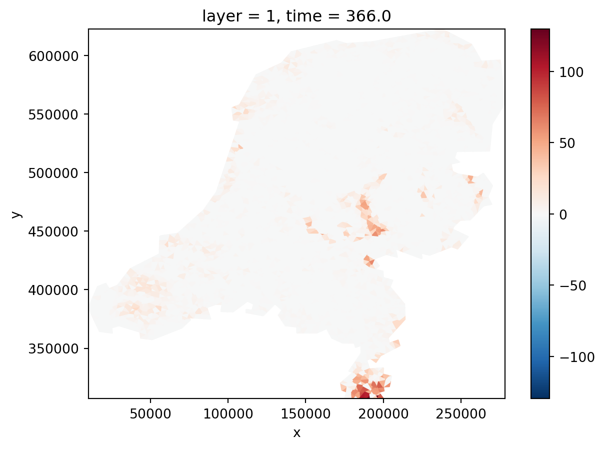

iMOD Python also supports partitioning a simulation, for parallel computation. It offers convenience functions to split existing simulations. For this we require a label array first.

from imod.prepare import create_partition_labels

label_array = create_partition_labels(idomain, npartitions=4)

label_array.ugrid.plot()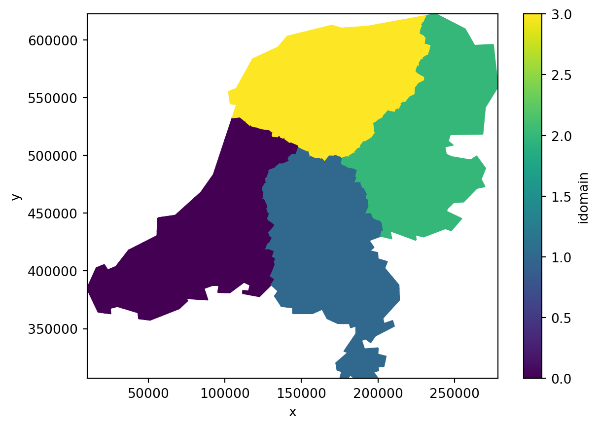

Let’s split our simulation with the label array.

simulation_split = simulation.split(label_array)

Now write the split simulation and run it

modeldir = tmpdir / "partitioned"
simulation_split.write(modeldir)
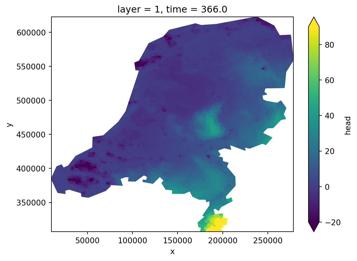
simulation_split.run(mf6_path)

And plot the results. Note that iMOD Python takes care of merging the 4 partitioned models into one single head grid.

head_merged = simulation_split.open_head()["head"].isel(time=-1, layer=0)
# plot
head_merged.ugrid.plot(vmin=-20, vmax=90)