MODFLOW 6 model for the Hondsrug

Note beforehand

This is a modified version of the Jupyter notebook distributed during the iMOD International days 2023. The modifications made to the original material mainly make accessing the data required for the course easier. To read the original course material follow this link.

Requirements

Python environment with iMOD Python version > 0.16.0
Start this notebook within a python environment where all required packages are installed. We suggest to use Deltaforge, a python distribution which includes iMOD Python and all its dependencies. Deltaforge is provided as an installer and makes installing iMOD Python easy. You can download the Deltaforge installer on the Deltares download portal.

Description

In this tutorial, you will learn how to use iMOD Python for building, running and analysing your MODFLOW 6 model. We compiled a tutorial to help you get started with iMOD Python and give you an overview of its capabilities.

In this Tutorial you learn how to: 1. load an existing model; 1. view some of the model input; 1. write and run the MODFLOW 6 simulation; 1. view results; 1. add a WEL package; 1. compare results; 1. replace the RCH package; 1. regrid the RCH package to the model dimensions.

We run this tutorial in a Jupyter notebook. You can run this cell by cell: [] means the cell is not run yet, [*] means the cell is currently running, [1] means the cell is finished. > Note: The cells where we run the simulation will take a few minutes.

Introduction case Hondsrug

The “Hondsrug” a Dutch ridge of sand over a range of 70 km. It is the only geopark in The Netherlands and part of Natura 2000, an European network of protected areas.

Start of the iMOD python tutorial

We’ll start off with importing iMOD Python. Therefore type import imod in the next cell and run it.

Code

import imod

From now on, all iMOD Python functions and classes are available. An important one is the class imod.mf6.Modflow6Simulation. An object from this class can contain one ore more complete MODFLOW 6 models. For more MODFLOW 6 functions and classes check the API Reference website

Read simulation from toml

With iMOD Python you can of course create a MODFLOW 6 model from scratch. It is also possible to read/import a model that was already created by iMOD Python. To share models iMOD Python uses a toml as configuration file and netcdf for data.
You find the toml file for this tutorial in the tutorial database named “… -hondsrug-example.toml”.

This is the content of the toml file:

[GroundwaterFlowModel]
  GWF = "GWF/GWF.toml"
[Solution]
  solver = "solver.nc"
[TimeDiscretization]
  time_discretization = "time_discretization.nc"

From this toml you see that in turn it refers to another toml for the content of ground water model GWF, in the section [GroundwaterFlowModel]. The toml contains solver settings in the section [Solution] and timing information in the section [TimeDiscretization].

We will use the function from_file to load this MODFLOW 6 model from the toml file. This returns a so called Modflow6Simulation object. We will show that this object behaves similar to a python dictionary.

NB With iMOD Python you can create native MODFLOW 6 model files (e.g. .dis6, .npf6, *.rch6 files). iMOD Python functions to read native MODFLOW 6 model files follow in 2024.

Read simulation from toml

iMOD Python shares Modflow 6 models using a toml and netcdf. Native Modflow 6 models can be written by the package, but not be read. You can use the from_file constructor method to load a simulation created with iMOD Python. This returns a Modflow6Simulation object, which behaves similar to a python dictionary. A Modflow6Simulation can contain multiple Groundwater Flow and Groundwater Transport models. In this example we’ll load the Modflow6Simulation directly from the data distributed with iMOD Python.

Code

tmpdir = imod.util.temporary_directory()

simulation = imod.data.hondsrug_simulation(tmpdir / "hondsrug_saved")

# Ensure xt3d is not used
simulation["GWF"]["npf"].set_xt3d_option(is_xt3d_used=False, is_rhs=False)

Downloading file 'hondsrug-simulation.zip' from 'https://github.com/Deltares/imod-artifacts/raw/main/hondsrug-simulation.zip' to '/home/runner/.cache/imod'.

The toml file is read and now the MODFLOW 6 model object is created. We stated that this object behaves like a python dictionary. Let’s have a look at the content. You can run print(simulation) or even simulation.

Code

simulation

Modflow6Simulation(
    name='mf6-hondsrug-example',
    directory=None
){
    'GWF': GroundwaterFlowModel,
    'solver': Solution,
    'time_discretization': TimeDiscretization,
}

In this overview you recognize the content of the toml file again. The groundwater model in this object is named “GWF”, we can access this model as follows.

Code

gwf_model = simulation["GWF"]

This returns the GroundwaterFlowModel object, which also behaves as a dictionary. This contains the package name as key, and a package object as value. We can print the content again with pretty print.

Code

gwf_model

GroundwaterFlowModel(
    listing_file=None,
    print_input=False,
    print_flows=False,
    save_flows=False,
    newton=False,
    under_relaxation=False,
){
    'dis': StructuredDiscretization,
    'npf': NodePropertyFlow,
    'ic': InitialConditions,
    'chd': ConstantHead,
    'rch': Recharge,
    'drn-pipe': Drainage,
    'riv': River,
    'sto': SpecificStorage,
    'oc': OutputControl,
}

Next step is to to access the data of a model package from the model object. In this example we access the data in the River package.

Code

riv_pkg = gwf_model["riv"]

This riv_pkg is just the river object. To actually access the data in this package, we use the dataset attribute. This returns an xarray Dataset which is the important data structure on which iMOD Python is built. If you want to read more about these objects, see the xarray documentation here.

Code

riv_pkg

You can see that it is indeed an xarray Dataset. You also see that this river package has data on three Dimensions: x, y and layer. From the Coordinates list you can read that there is data defined on 4 layers, namely: 1, 3, 5, 6.
The Data variables section show that data is available for the 3 parameters required for the river package: “stage”, “conductance” and “bottom_elevation”.

By the way, what is actually the number of layers in our model?
From all MODFLOW 6 packages, only DIS, NPF and STO are defined for all layers. So in one of those packages you find your answer.
Assignment: “Find the total number of layers in our model from one of these packages”

Code

# type your command here.....

Now we return to our river package, available in “riv_pkg”. We can select the stage information in layer 1 as follows:

select variable “stage” from the Dataset;
and select only the “stage” values for the 1st layer.

Code

riv_stage_layer_1 = riv_pkg["stage"].sel(layer=1)

The result is a 2 dimensional (x/y) xarray Dataset. We can have a look at the content by just typing the object name.

Code

riv_stage_layer_1

Plot model parameters

An xarray Dataset has plot functionalities included. This makes it easy to get an impression of the spatial distrubution of our stage values for layer 1.
In the next cell just type the name of 2D Dataset you just created including the call for the plot function .plot(). %% replace with your plot command

Congratulations, your first picture in this tutorial!
Instead of this default plot option, we can plot this stage data also on a map with the iMOD Python function imod.visualize.plot_map.

We’ll start off by defining a colormap and levels for the legend.

Code

import numpy as np

colors = "Blues"
levels = np.arange(-2.5, 18.5, 2.5)

With this colormap, the legend range and the 2d Dataset, we call the iMOD Python plot_map function:

Code


imod.visualize.plot_map(riv_stage_layer_1, colors, levels)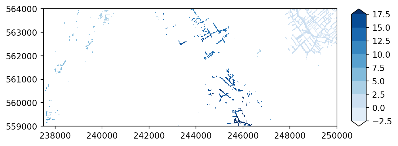

As you can see imod.visualize.plot_map preserves the aspect ratio, whereas the .plot method stretches the figure in the y-direction to make a square figure.

Try plotting with a different colormap. For all possible colormaps, see the Matplotlib page. For instance pick colormap “viridis”.

Code

colors = "viridis"  # specify your color here

imod.visualize.plot_map(riv_stage_layer_1, colors, levels)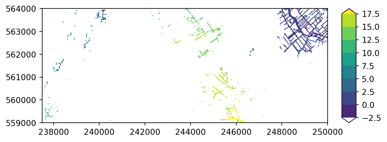

We can add a background map to this plot for a better orientation. Therefore we need to import the package contextily first. This opens a wide range of possible basemaps, see the full list here. * Next step is to define our background_map, in this example it is one of the OpenStreetMap variants. * The we add this basemap as argument to our plot function.

Code

import contextily as ctx

# Access background maps
background_map = ctx.providers["OpenStreetMap"]["Mapnik"]

# Add background map to your plot
imod.visualize.plot_map(riv_stage_layer_1, colors, levels, basemap=background_map)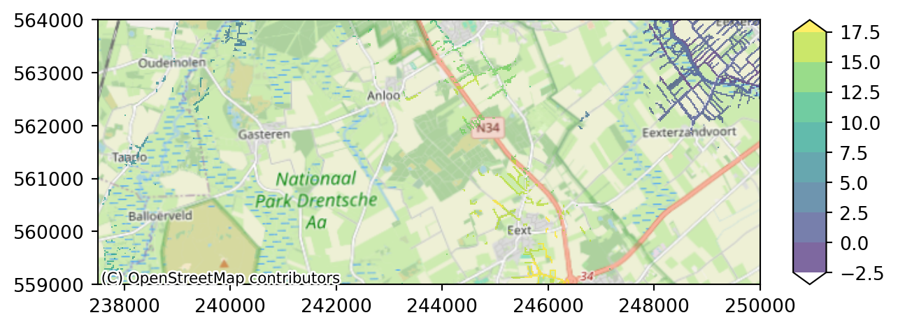

Assignment: in the next cell, try to visualize the bottom elevation of layer 3.

Code

#
# type here you python commands to select and plot bottom data for layer 3

It can be convenient to combine the rivers over all layers into one map. You can aggregate layers using xarrays aggregation functionality. For example we can compute the mean of the river stage across all layers:

Code

riv_all = riv_pkg["stage"].mean(dim="layer")

imod.visualize.plot_map(riv_all, colors, levels, basemap=background_map)

Running the simulation

Now it’s time to run the MODFLOW 6 simulation. 1. First we create a result folder. 1. Then we write the MODFLOW 6 input file, so the mfsim.nam file and all other package input files 1. Finally we run the model with the MODFLOW 6 executable. Now it’s time to run the simulation. This takes a few minutes.

Step 1. To create a result folder, we will import the package pathlib first. The name of the result folder for this initial model is “reference”.

Code

# Define the project directory where you want to write and run the Modflow 6
# simulation.
prj_dir = tmpdir / "results"

modeldir = prj_dir / "reference"

Step 2. You remember the MODFLOW 6 model object “simulation” that contained our full MODFLOW 6 model. This object has the function .write. The function converts the model to native MODFLOW 6 input files, so the mfsim.nam file and all other package files like .dis, .drn and *.riv.

Code

# Write the MODFLOW 6 simulation files from the model object
simulation.write(modeldir)

In your file manager check if the MODFLOW 6 files are created in your result folder, e.g. NAM file “c:\2023.nam”

Step 3 is to run the run our model with the MODFLOW 6 executable. Therefore we use the function .run from our model object “simulation”. The only parameter is the path name of the MODFLOW 6 executable.

NB Before you run the simulation, provide the function the correct path to the MODFLOW 6 executable.
NB The run takes a few minutes.

Code

# mf6_path = "path/to/mf6.exe" 

# If you installed Modflow6 in your PATH environment variable, you can use the
# following argument:
mf6_path = "mf6"

simulation.run(mf6_path)

Exploring the results

We can open the heads with the .open_head method. This automatically finds the appropriate files to open the model output.

The calculated heads are saved in the file “GWF/GWF.hds”. In order to display these results spatially correct, the values must be plotted on the corrrect grid topology. The grid of our model is available in the Binary Grid file “GWF/dis.dis.grb”.

Code

calculated_heads = simulation.open_head()

Let’s check the content of this xarray Dataset.

Code

calculated_heads

<xarray.DataArray 'head' (time: 7, layer: 13, y: 200, x: 500)> Size: 73MB
dask.array<stack, shape=(7, 13, 200, 500), dtype=float64, chunksize=(1, 13, 200, 500), chunktype=numpy.ndarray>
Coordinates:
  * x        (x) float64 4kB 2.375e+05 2.375e+05 2.376e+05 ... 2.5e+05 2.5e+05
  * y        (y) float64 2kB 5.64e+05 5.64e+05 5.639e+05 ... 5.59e+05 5.59e+05
    dx       float64 8B 25.0
    dy       float64 8B -25.0
  * layer    (layer) int64 104B 1 2 3 4 5 6 7 8 9 10 11 12 13
  * time     (time) float64 56B 1.157e-05 365.0 730.0 ... 1.826e+03 2.191e+03

This dataset contains calculated heads for all 13 layers. For the first time we see that our full model contains also 7 stress periods: time:7.
We can select heads for all layers at the final timestep with the .isel function, meaning a selection based on index number.

Code

heads_end = calculated_heads.isel(time=-1)

heads_end

<xarray.DataArray 'head' (layer: 13, y: 200, x: 500)> Size: 10MB
dask.array<getitem, shape=(13, 200, 500), dtype=float64, chunksize=(13, 200, 500), chunktype=numpy.ndarray>
Coordinates:
  * x        (x) float64 4kB 2.375e+05 2.375e+05 2.376e+05 ... 2.5e+05 2.5e+05
  * y        (y) float64 2kB 5.64e+05 5.64e+05 5.639e+05 ... 5.59e+05 5.59e+05
    dx       float64 8B 25.0
    dy       float64 8B -25.0
  * layer    (layer) int64 104B 1 2 3 4 5 6 7 8 9 10 11 12 13
    time     float64 8B 2.191e+03

Let’s plot the heads for layer 3 only. Use the function .plot_map as we did before. Be aware that instead of using the .isel function, we now use .sel. Within xarray this is a selection based on index name instead of index numer.

Code

imod.visualize.plot_map(heads_end.sel(layer=3), colors, levels, basemap=background_map)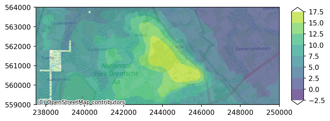

As you can see layer 3 has some missing cells in the west. Whereas layer 4 only contains active cells in the eastern peatland area.

Assignment: add your plot command for layer 4 in the cell below.

Code

# type your command here.....
# TODO remove example
imod.visualize.plot_map(heads_end.sel(layer=5), colors, levels, basemap=background_map)

Layer 5 contains more data towards the west, but has no active cells in the centre.

Code

# type your command here.....
# TODO remove example
imod.visualize.plot_map(heads_end.sel(layer=5), colors, levels, basemap=background_map)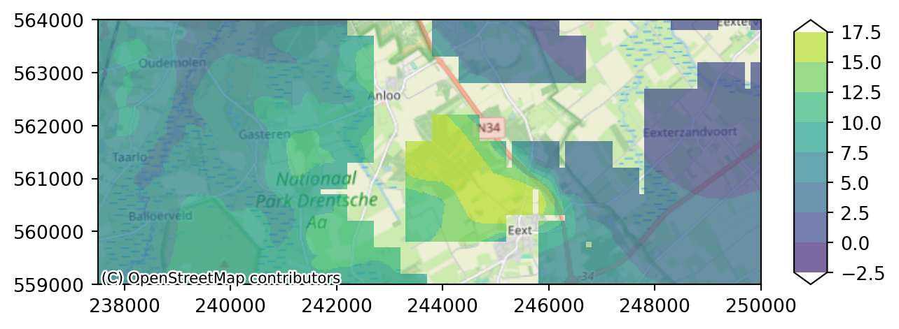

As you can see the data is individual layers have lots of inactive cells in different places. It is difficult for this model to get a good idea what is happening across the area based on 1 layer alone. Luckily xarray allows us to compute the mean across a selection of layers by first selecting 3 layers (first aquifer) with .sel, and then computing the mean across the layer dimension.

We can do that in 2 lines of code:
head_end_3layers = heads_end.sel(layer=slice(3, 5))
head_end_aq1 = head_end_3layers.mean(dim="layer")
Or we can concatenate both steps to one:

Code

head_end_aq1 = heads_end.sel(layer=slice(3, 5)).mean(dim="layer")

imod.visualize.plot_map(head_end_aq1, colors, levels, basemap=background_map)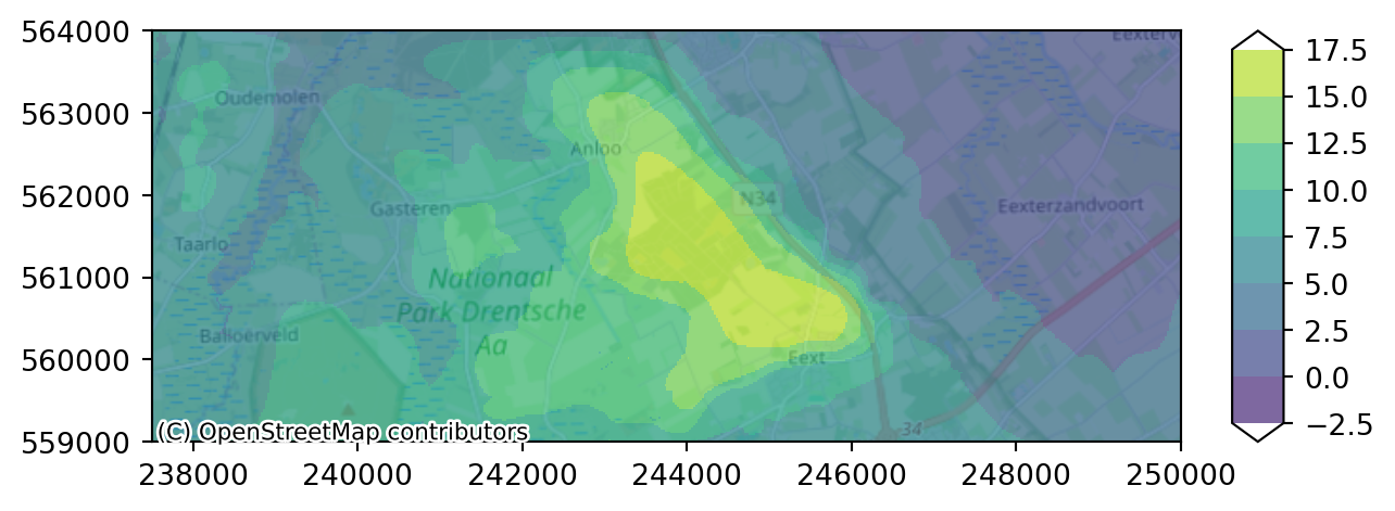

Adding a well

Let’s add an extraction well at x=246000 and y=560000. Therefore we create a well object first. We use variables x_well and y_well to define the location so we can reuse the variables later on. We can provide a well screen top and bottom and iMOD Python automatically places the well in the right layer(s) upon writing the model.

Code

x_well = 246000.0
y_well = 560000.0
# create a well object
well = imod.mf6.Well(
    screen_top=[-13.0],
    screen_bottom=[-50.0],
    y=[y_well],
    x=[x_well],
    rate=[-60000.0],
)

Next step is to add your well (object) to the existing groundwater model “GWF”.

Code

simulation["GWF"]["wel"] = well

Interested to see if the package was added correctely?
Get the list of available package by adding the command gwf_model in the cell above and run the cell again.

We are ready to rerun the model and check the drawdown effect of the well. Do you recall the steps we took in order to get the mean head for layers 1 to 3?
Step 1: define the result folder and run the model.
Step 2: read the calculated heads.
Step 3: select the last stressperiod and average over layers 1 to 3.

In the next cell, give this scenario run a name:

Code

# Step 1: run the model
modeldir = prj_dir / "extraction"
simulation.write(modeldir)
simulation.run(mf6_path)

Code

# Step 2: export the calculated heads

heads_with_well = simulation.open_head()

heads_with_well

<xarray.DataArray 'head' (time: 7, layer: 13, y: 200, x: 500)> Size: 73MB
dask.array<stack, shape=(7, 13, 200, 500), dtype=float64, chunksize=(1, 13, 200, 500), chunktype=numpy.ndarray>
Coordinates:
  * x        (x) float64 4kB 2.375e+05 2.375e+05 2.376e+05 ... 2.5e+05 2.5e+05
  * y        (y) float64 2kB 5.64e+05 5.64e+05 5.639e+05 ... 5.59e+05 5.59e+05
    dx       float64 8B 25.0
    dy       float64 8B -25.0
  * layer    (layer) int64 104B 1 2 3 4 5 6 7 8 9 10 11 12 13
  * time     (time) float64 56B 1.157e-05 365.0 730.0 ... 1.826e+03 2.191e+03

Code

# Step 3: select the last stressperiod and average over layers 1 to 3.
heads_with_well_end = heads_with_well.isel(time=-1)
heads_with_well_end_aq1 = heads_with_well_end.sel(layer=slice(3, 5)).mean(dim="layer")

Compute differences

Let’s compare differences between the two scenarios, by computing difference in heads and plot this on a map.

Code

# Calculate the head difference.
diff = heads_with_well_end_aq1 - head_end_aq1

Plot the result

Code


colors = "Blues"
levels = np.arange(-2.5, 18.5, 2.5)

imod.visualize.plot_map(diff, colors, levels, basemap=background_map)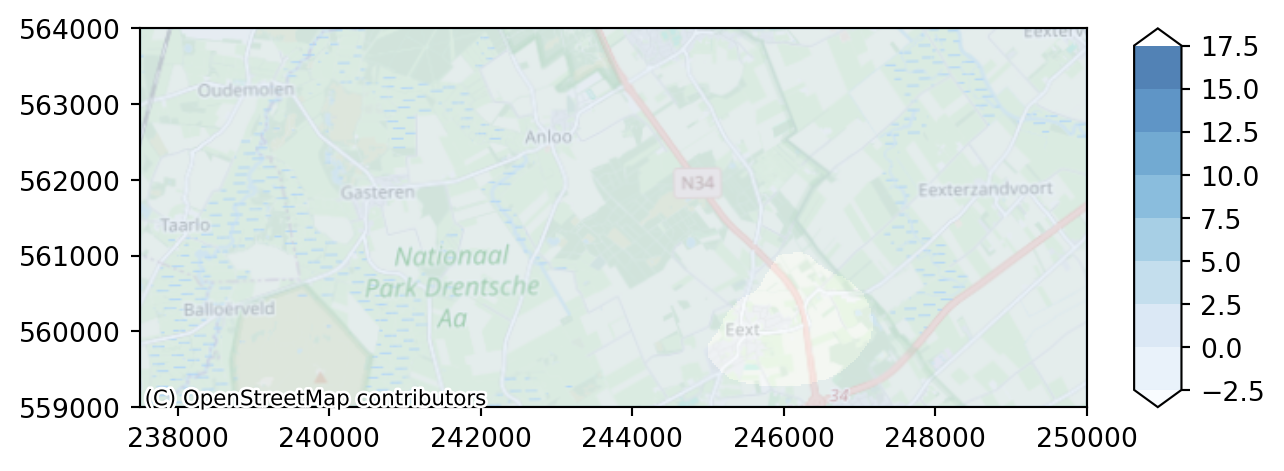

With this legend, we can not see the impact of the well effect enough. We need another legend; both anouther color range and another range of values.
Assignment: - make the levels range from -10 to 0 meter with steps of 1 meter. - choose “hot” for colorbar

Code

# levels = ?
# colors = ?
# TODO: onderstaande regels verwijderen
levels = np.arange(-10.0, 0.0, 1.0)
colors = "hot"
imod.visualize.plot_map(diff, colors, levels, basemap=background_map)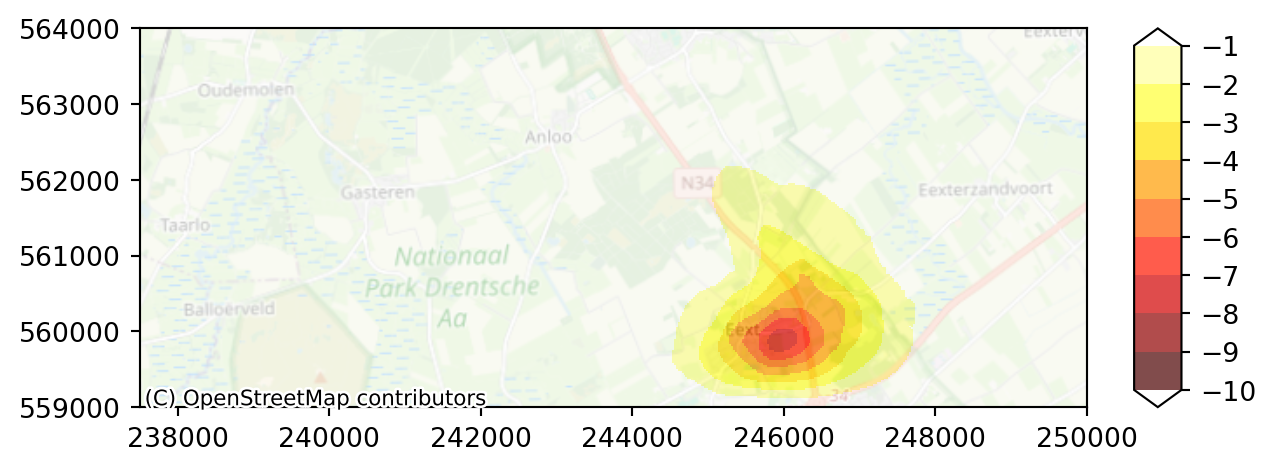

Adding recharge

The model read from the toml file contains already some transient recharge that we are going to replace. But first check the figure below and see the mean at 31 December 2014.

figure: mean recharge on 31-12-2014

Do you think you can plot this figure yourself now you have some experience?
Assignment: apply correct methods for time and layer to the dataset simulation["GWF"]["rch"]["rate"] and plot your figure.

Code

# add functions
# simulation["GWF"]["rch"]["rate"]..........

Now we open the dataset with the xarray function into variable ‘meteorology’.

Code

meteorology = imod.data.hondsrug_meteorology()

Downloading file 'hondsrug-meteorology.nc' from 'https://github.com/Deltares/imod-artifacts/raw/main/hondsrug-meteorology.nc' to '/home/runner/.cache/imod'.

Next step is to check the content of the dataset. See that is contains spatial data from 1999-01-01 till 2020-04-09.
For which 2 variables data is stored in the file?

Code

meteorology

Code

# A plot of the evapotranspiration at 202-04-09.
meteorology.isel(time=-1)["evapotranspiration"].plot()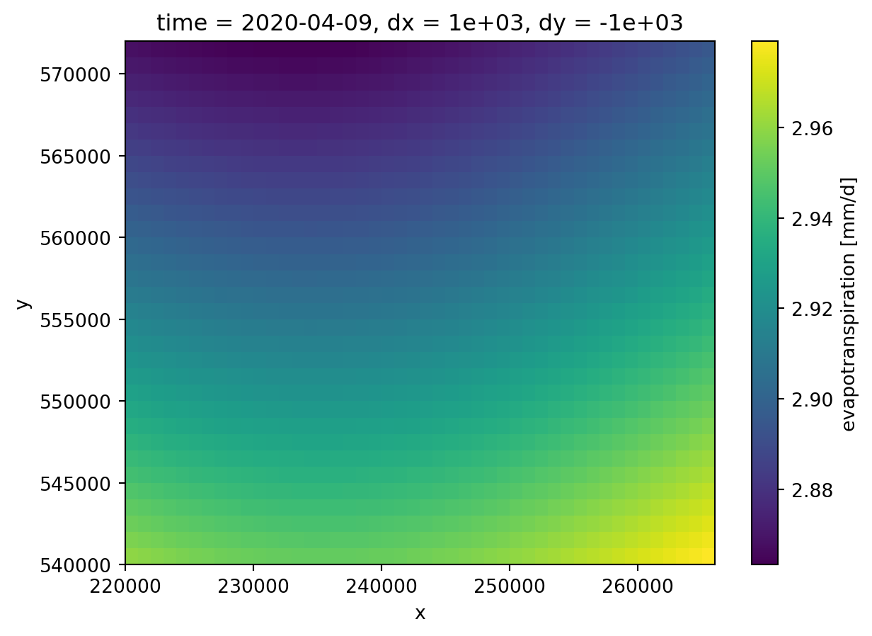

If you look carefully, you can see that the unit of this dataset is in mm/d. Our MODFLOW 6 model is defined in m/d, so we’ll have to convert units here. Xarray allows you to do computations on complete datasets, so we can divide both the precipitation and the evapotranspiration by 1000.0.

Code

meteorology = meteorology / 1000.0

For your own reference (and your colleagues), it is wise to update the units in the attributes of the dataset

Code

meteorology.attrs["units"] = "m/d"

meteorology

We’ll compute the recharge very rudimentarily by subtracting the precipitation from the evapotranspiration.

Code

recharge = meteorology["precipitation"] - meteorology["evapotranspiration"]

For the steady state conditions of the model, the data from the period 2000 to 2009 is considered as reference. The initial information must be sliced to this time period and averaged to obtain the a mean value grid.

Assignment: fill in the start and end data for our reference period using yyyy-mm-dd.

Code

# slice recharge based on date
recharge_first_decade = recharge.sel(time=slice("2000-01-01", "2009-12-31"))
# calculate the steady state recharge
recharge_steady_state = recharge_first_decade.mean(dim="time")

Code

# redefine the legend values
levels = np.arange(0.0, 0.0011, 1e-4)

# plot with color bar "blues"
imod.visualize.plot_map(recharge_steady_state, "Blues", levels, basemap=background_map)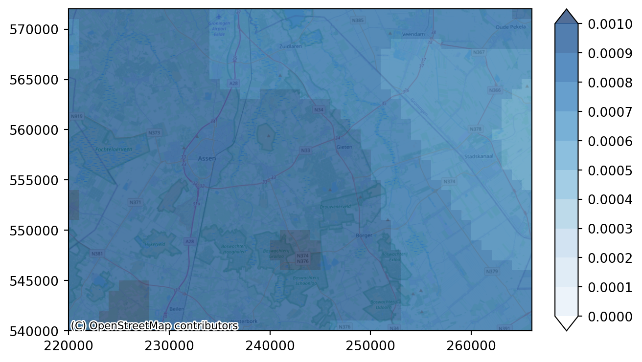

Finding the right levels for this plot can be cumbersome. So we can define a function to compute appropriate levels for the plot based on a given DataArray and a desired number of legend levels.

Code

def compute_levels(da, N):
    """
    This function computes N levels based on the range of a provided DataArray "da".

    Parameters
    ----------
    da: xr.DataArray
        The DataArray for which a number of levels needs to be computed
    N: int
        The number of levels
    """
    levels = np.linspace(da.min(), da.max(), N)
    return levels


# call to the function for a 10 level legend
levels = compute_levels(recharge_steady_state, 10)
# plot the recharge figure
imod.visualize.plot_map(recharge_steady_state, "Blues", levels, basemap=background_map)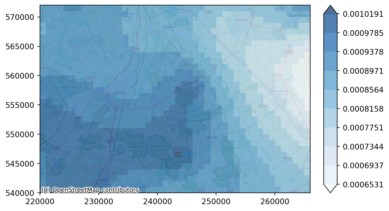

Aligning the recharge data over time

The recharge data has quite a lot of timesteps: data on a daily timestep for over 20 years from 1999 to 2020.

Code

recharge.coords["time"]

This is entirely different from our model discretization as you can see from the next command. It is on a yearly timestep and lasts from 2010 to 2015.

Code

simulation["time_discretization"]["time"]

<xarray.DataArray 'time' (time: 7)> Size: 56B
array(['2009-12-30T23:59:59.000000000', '2009-12-31T00:00:00.000000000',
       '2010-12-31T00:00:00.000000000', '2011-12-31T00:00:00.000000000',
       '2012-12-31T00:00:00.000000000', '2013-12-31T00:00:00.000000000',
       '2014-12-31T00:00:00.000000000'], dtype='datetime64[ns]')
Coordinates:
  * time     (time) datetime64[ns] 56B 2009-12-30T23:59:59 ... 2014-12-31

We therefore need to align this data over time. We’ll start off by selecting the data in this time range.

Code

recharge_daily = recharge.sel(time=slice("2010-01-01", "2015-12-31"))

recharge_daily

Xarray has functionality to resample recharge to yearly timestep (“A” stands for “annum”). If you want to find the aliases for other frequencies, see this table We’ll label the years with their starting point, as iMOD Python defines its stress periods on their starting moment.

Code

recharge_yearly = recharge_daily.resample(time="A", label="left").mean()

recharge_yearly

To visually compare the effects of the yearly versus daily recharge, we can make a lineplot. For there plot functionalities we need to import the package matplotlib one-time. We’ll take a point close to the well. We can use:

Code

import matplotlib.pyplot as plt

# initialization of the figure and single graph
fig, ax = plt.subplots()
# defining the content of the graph
recharge_daily.sel(x=x_well, y=y_well, method="nearest").plot(ax=ax)
recharge_yearly.sel(x=x_well, y=y_well, method="nearest").plot(ax=ax)
# display the graph
plt.show()

To create the final recharge for the transient simulation, the steady state information needs to be concatenated to the transient recharge data. The steady state simulation will be run for one second. This is achieved by using the numpy Timedelta function, first creating a time delta of 1 second, which is assigned to the steady-state recharge information. This dataset is then concatenated using the xarray function xarray.concat to the transient information and indicating that the dimension to join is "time".

Code

import xarray as xr

starttime = "2009-12-31"

# create second before transient
one_second = np.timedelta64(1, "s")  # 1 second duration for initial steady-state
starttime_ss = np.datetime64(starttime) - one_second
# fill in with steady-state value
recharge_steady_state = recharge_steady_state.assign_coords(time=starttime_ss)
# add before transient data
recharge_ss_yearly = xr.concat([recharge_steady_state, recharge_yearly], dim="time")
# check timesteps
recharge_ss_yearly.coords["time"]

/tmp/ipykernel_5017/3227820086.py:9: UserWarning: Converting non-nanosecond precision datetime values to nanosecond precision. This behavior can eventually be relaxed in xarray, as it is an artifact from pandas which is now beginning to support non-nanosecond precision values. This warning is caused by passing non-nanosecond np.datetime64 or np.timedelta64 values to the DataArray or Variable constructor; it can be silenced by converting the values to nanosecond precision ahead of time.
  recharge_steady_state = recharge_steady_state.assign_coords(time=starttime_ss)

The Recharge package requires a layer coordinate to assign values to. We’ll assign all values to the first layer.

Code

recharge_ss_yearly = recharge_ss_yearly.assign_coords(layer=1)
# see that coordinate "layer" is added
recharge_ss_yearly

Furthermore, iMOD Python expects its data to follow the dimension order: ["time", "layer", "y", "x"]. The recharge data has order ["y", "x", "time"] after concatenation.

Code

recharge_ss_yearly = recharge_ss_yearly.transpose("time", "y", "x")

recharge_ss_yearly

We’ll assign the recharge to recharge package.

Code

recharge_pkg_coarse = imod.mf6.Recharge(rate=recharge_ss_yearly)

recharge_pkg_coarse

This recharge package is defined on a coarse grid and not the model grid. iMOD Python has functionality regrid_like to regrid model packages to the appropriate grid. We’ll use the first layer of the idomain in our model as the template grid.

Note that we create a RegridderWeightsCache here. This will store the weights of the regridder. Using the same cache to regrid another package will lead to a performance increase if that package uses the same regridding method, because initializing a regridder is costly.

Code

from imod.mf6.utilities.regrid import RegridderWeightsCache

template_grid = gwf_model["dis"]["idomain"].sel(layer=1)

regrid_context = RegridderWeightsCache(recharge_ss_yearly.isel(time=0), template_grid)
recharge_pkg = recharge_pkg_coarse.regrid_like(template_grid, regrid_context)

recharge_pkg

MODFLOW 6 does not accept recharge cells which are assigned to inactive cells (where idomain != 1). iMOD Python therefore has convenience functions to get the upper active layer

Code

from imod.prepare import get_upper_active_grid_cells

# Select the grid cells where idomain == 1, these are the active cells.
idomain = gwf_model["dis"]["idomain"]
is_active = idomain == 1
# Find the upper active cells
is_upper_active_grid = get_upper_active_grid_cells(is_active)
# We can use xarrays where method to broadcast the recharge rates to the upper
# active cells.
recharge_pkg["rate"] = recharge_pkg["rate"].where(is_upper_active_grid)
# Finally reorder the dimensions of the dataset to how it is expected by iMOD
# Python.
recharge_pkg.dataset = recharge_pkg.dataset.transpose("time", "layer", "y", "x")

recharge_pkg

We’ll override the recharge package with our newly computed recharge package

Code

gwf_model["rch"] = recharge_pkg

Write the simulation and run it again

Code

modeldir = prj_dir / "new_recharge"
simulation.write(modeldir)
simulation.run(mf6_path)

Code

# Open heads
head_new_recharge = simulation.open_head()

head_new_recharge

<xarray.DataArray 'head' (time: 7, layer: 13, y: 200, x: 500)> Size: 73MB
dask.array<stack, shape=(7, 13, 200, 500), dtype=float64, chunksize=(1, 13, 200, 500), chunktype=numpy.ndarray>
Coordinates:
  * x        (x) float64 4kB 2.375e+05 2.375e+05 2.376e+05 ... 2.5e+05 2.5e+05
  * y        (y) float64 2kB 5.64e+05 5.64e+05 5.639e+05 ... 5.59e+05 5.59e+05
    dx       float64 8B 25.0
    dy       float64 8B -25.0
  * layer    (layer) int64 104B 1 2 3 4 5 6 7 8 9 10 11 12 13
  * time     (time) float64 56B 1.157e-05 365.0 730.0 ... 1.826e+03 2.191e+03

Code


diff_new_rch = head_new_recharge - calculated_heads

diff_new_rch_end_first_aqf = (
    diff_new_rch.isel(time=-1).sel(layer=slice(3, 5)).mean(dim="layer")
)

levels = np.arange(-10.0, 0.0, 1.0)

imod.visualize.plot_map(
    diff_new_rch_end_first_aqf, "hot", levels, basemap=background_map
)

Create a cross-section

Making a cross-section is rather easy in iMOD Python. We can use the function imod.select.cross_section_linestring. Furthermore we only need gridded data and a line to slice through the data. For this tutorial let’s make a cross-section and display the permeability of the layers. * First we create a geology data set with the “permeability” and of course the ‘top’ and ‘bottom’ of all the layers. * Then we slice the data set with a line and plot the result.

Create geology dataset

The “permeability” of the model is available in the “npf” package of our model. So we start to fill a new “geology” dataset with this “k” value.

Code

geology = gwf_model["npf"]["k"]

The “top” and “bottom” information of layers is available in the “dis” package. Unfortunately the “dis” package has bottom information for all layers but only top information for layer 1. Check this in the next cell.

Code

gwf_model["dis"]

So first we add the bottom information to our geology dataset.

Code

geology["bottom"] = gwf_model["dis"]["bottom"]

Then we define the top of layer 1 to be the Digital Elevation Model (DEM). Next, for layer 2 to 13, we must fill in the top of each layer with the bottom of the layer above (e.g. top_l5 = bot_l4). Seems like a bit complicated? No, we can use the .shift function of xarray for this.

Code

DEM = gwf_model["dis"]["top"]
geology["top"] = geology["bottom"].shift(layer=1).fillna(DEM)

# Check the content of geology data set
geology

Let’s plot the top of our model, the DEM.

Code

levels = compute_levels(DEM, 10)
imod.visualize.plot_map(DEM, "viridis", levels, basemap=background_map)

Plot cross-section

The geology is ready so the last element we need is the cross-section line. In the data set the Esri Shape “crosssection.shp” is available. We need the package geopandas to read the file into a GeoDataFrame object.

Code


crossline = imod.data.hondsrug_crosssection(tmpdir / "cross-section")

Downloading file 'hondsrug-crosssection.zip' from 'https://github.com/Deltares/imod-artifacts/raw/main/hondsrug-crosssection.zip' to '/home/runner/.cache/imod'.

We can plot our DEM again and add our cross-section line as an overlay to our function plot_map.

Code

# define overlay
overlays = [{"gdf": crossline, "edgecolor": "black",  "linewidth":3}]
# Plot
imod.visualize.plot_map(DEM, "viridis", levels, overlays, basemap=background_map)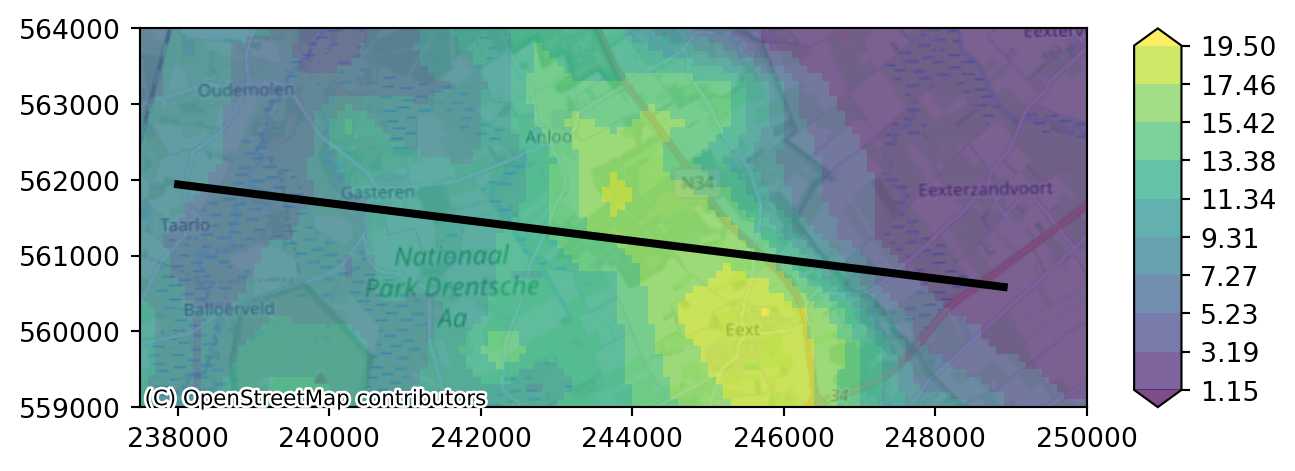

In the next cell we call the function cross_section_linestring together with our geology dataset and the geometry of our line. The result is a 2D DataArray “cross_k” with k-values along the line for all layers. We can plot this DataArray with the visualization function cross_section.

Code

cross_k = imod.select.cross_section_linestring(geology, crossline.geometry[0])
levels = np.arange(0.0, 30.0, 5)
colors = "viridis"
imod.visualize.cross_section(cross_k, colors, levels)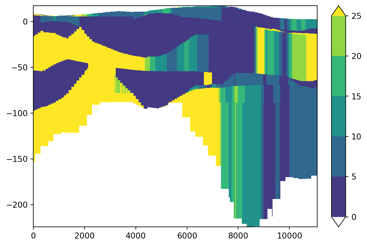

With the package shapely you can easily make new geometries by hand for displaying other cross-sections. The next example is a new line from North to South over the area. You can play around with lines, colors and levels.

Code

from shapely.geometry import LineString

geometry = LineString([[244000,563000],[244000 ,559000]])
cross_k = imod.select.cross_section_linestring(geology, geometry)
imod.visualize.cross_section(cross_k, colors, levels)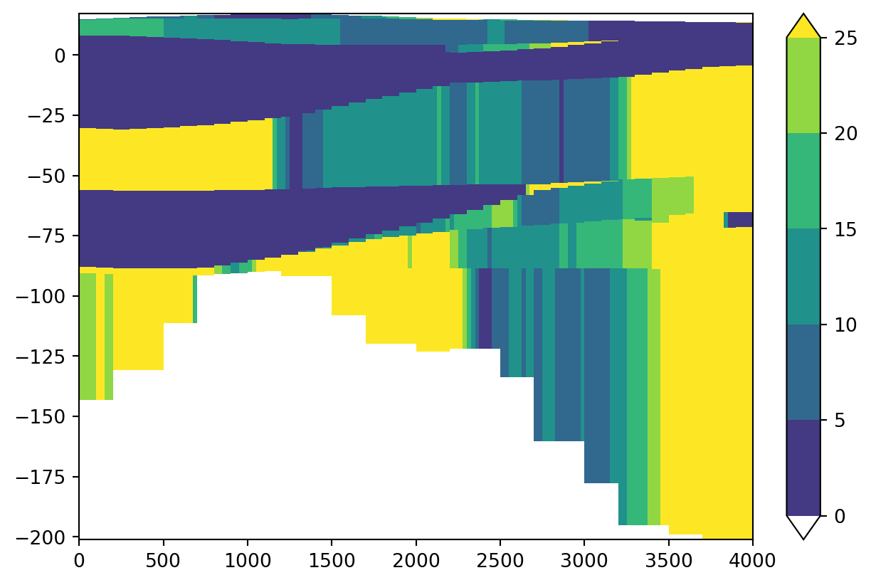

Model partitioning

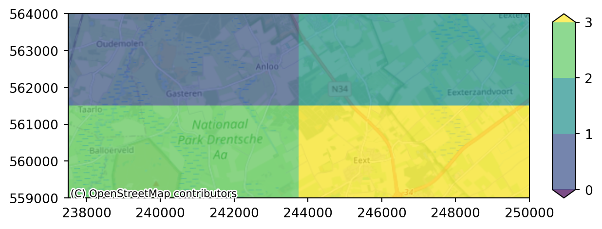
We can partition our simulation into multiple sub-models. This is useful for parallel computation. We need to specify the different domains to iMOD Python by providing a grid with each subdomain labeled with a unique number. To create 4 submodels (required to compute on 4 cores in parallel), we can manually create this grid as follows:

Code


from imod.mf6.multimodel.partition_generator import get_label_array

npartitions = 4
submodel_labels = get_label_array(simulation, npartitions=npartitions)


# Plot the submodel labels
label_levels = np.arange(npartitions)

imod.visualize.plot_map(
    submodel_labels,
    "viridis",
    label_levels,
    basemap=background_map,
)

We consequently partition our simulation as follows with the split function:

Code

simulation_split = simulation.split(submodel_labels)

simulation_split

Modflow6Simulation(
    name='mf6-hondsrug-example_partioned',
    directory=None
){
    'solver': Solution,
    'time_discretization': TimeDiscretization,
    'GWF_0': GroundwaterFlowModel,
    'GWF_1': GroundwaterFlowModel,
    'GWF_2': GroundwaterFlowModel,
    'GWF_3': GroundwaterFlowModel,
    'split_exchanges': list,
}

Notice the presence of the 4 groundwater flow models! Let’s run them:

Code

modeldir = prj_dir / "partitioning"
simulation_split.write(modeldir)
simulation_split.run(mf6_path)

Modflow 6 writes heads for each partition seperately. It is more convenient to merge these heads into one grid again, which we can compare with the original grid. Luckily, the open_head function automatically merges heads for us.

Code

head_split = simulation_split.open_head()["head"]

head_split

<xarray.DataArray 'head' (time: 7, layer: 13, y: 200, x: 500)> Size: 73MB
dask.array<concatenate, shape=(7, 13, 200, 500), dtype=float64, chunksize=(1, 13, 200, 500), chunktype=numpy.ndarray>
Coordinates:
  * x        (x) float64 4kB 2.375e+05 2.375e+05 2.376e+05 ... 2.5e+05 2.5e+05
  * y        (y) float64 2kB 5.64e+05 5.64e+05 5.639e+05 ... 5.59e+05 5.59e+05
    dx       float64 8B 25.0
    dy       float64 8B -25.0
  * layer    (layer) int64 104B 1 2 3 4 5 6 7 8 9 10 11 12 13
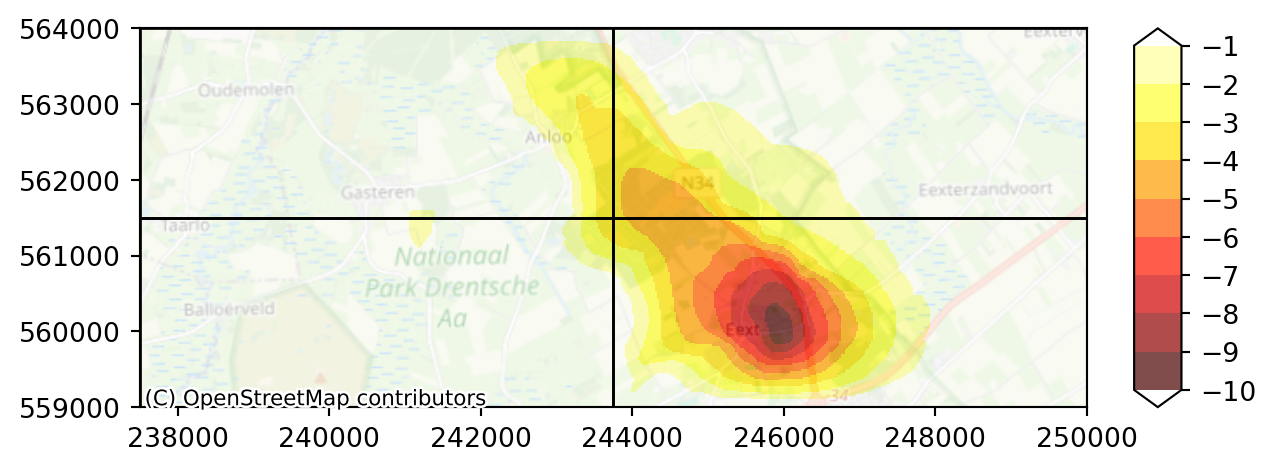
  * time     (time) float64 56B 1.157e-05 365.0 730.0 ... 1.826e+03 2.191e+03

For the final plot, it is good to have the submodel partitions as an overlay over our plot. The plot_map function has an overlays argument which we can use to plot overlays on our map. See also this example how you can apply this. This requires polygons though, and we have a raster. We can polygonize our raster with the imod.prepare.polygonize utility function:

Code

submodel_polygons = imod.prepare.polygonize(submodel_labels)

submodel_polygons

	value	geometry
0	0.0	POLYGON ((237500.000 564000.000, 237500.000 56...
1	1.0	POLYGON ((243750.000 564000.000, 243750.000 56...
2	2.0	POLYGON ((237500.000 561500.000, 237500.000 55...
3	3.0	POLYGON ((243750.000 561500.000, 243750.000 55...

Next we will plot the splitted output same as before. Notice that we have to provide the overlays with a dictionary, in which we can specify some extra settings. In this case, we do not want the polygons colored, but only the edges of the polygons colored. We can do this as follows:

Code

overlays = [{"gdf": submodel_polygons, "edgecolor": "black", "facecolor": "None"}]

diff_split = head_split - calculated_heads

diff_split_end_first_aqf = (
    diff_split.isel(time=-1).sel(layer=slice(3, 5)).mean(dim="layer")
)

levels = np.arange(-10.0, 0.0, 1.0)

imod.visualize.plot_map(
    diff_split_end_first_aqf, "hot", levels, basemap=background_map, overlays=overlays
)

Extra exercise

The yearly recharge did not differ much over time. Try computing your model on monthly timestep below!

Code


fig, ax = plt.subplots()
# defining the content of the graph
recharge_daily.sel(x=x_well, y=y_well, method="nearest").plot(ax=ax)
recharge_yearly.sel(x=x_well, y=y_well, method="nearest").plot(ax=ax)
# display the graph
plt.show()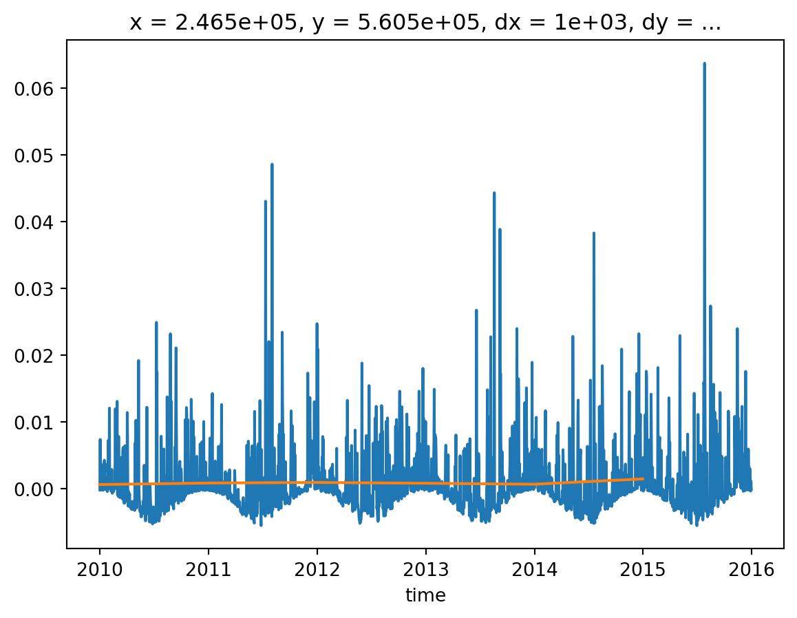

Tips

You can use the resample method to go from daily recharge to monthly recharge.
The table with aliases for frequencies can be found here.
Follow the consequent steps you did previously on your dataset to construct a Recharge package accepted by iMOD Python.
You have to create a new time discretization for your simulation, as the original simulation has yearly stress periods. You can use the create_time_discretization method for this.