Tip

For an interactive online version click here:

Plot DELWAQ data

HydroMT provides a simple interface to model schematization from which we can make beautiful plots:

• Raster layers are saved to the model grid attribute as a xarray.Dataset

• Vector layers are saved to the model geoms attribute as a geopandas.GeoDataFrame. Note that in case of DELWAQ these are not used by the model engine, but only for analysis and visualization purposes.

• Extracts from the linked hydrologic/hydraulic/hydrodynamic model are saved to the model hydromaps attribute as xarray.Dataset. In the case of DELWAQ they are not used by the engine but can be useful for post-processing.

We use the cartopy package to plot maps. This packages provides a simple interface to plot geographic data and add background satellite imagery.

Load dependencies

import numpy as np
import matplotlib.pyplot as plt

from hydromt_delwaq import DelwaqModel, DemissionModel

Read the model

root = 'EM_piave'
mod = DemissionModel(root, mode='r')
# Or for a DelwaqModel:
# mod = DelwaqModel('WQ_piave', mode='r')

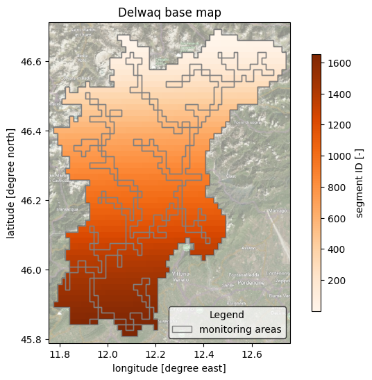
Plot model schematization base maps

Here we plot the model basemaps (Segment ID map with basins, monitoring points and areas geometries).

# plot maps dependencies
import matplotlib.patches as mpatches
import cartopy.crs as ccrs
import cartopy.io.img_tiles as cimgt

# read and mask the model elevation
da = mod.hydromaps['ptid'].raster.mask_nodata()
da.attrs.update(long_name='segment ID', units='-')
# read/derive model basin boundary
gdf_bas = mod.basins

nodata value missing for /home/runner/work/hydromt_delwaq/hydromt_delwaq/docs/_examples/EM_piave/hydromodel/rivarea.tif

# we assume the model maps are in the geographic CRS EPSG:4326
proj = ccrs.PlateCarree()
# adjust zoomlevel and figure size to your basis size & aspect
zoom_level = 10
figsize=(8, 6)
shaded= False # shaded elevation (looks nicer with more pixels (e.g.: larger basins))!


# initialize image with geoaxes
fig = plt.figure(figsize=figsize)
ax = fig.add_subplot(projection=proj)
extent = np.array(da.raster.box.buffer(0.02).total_bounds)[[0, 2, 1, 3]]
ax.set_extent(extent, crs=proj)

# add sat background image
ax.add_image(cimgt.QuadtreeTiles(), zoom_level, alpha=0.5)

## plot ptid
cmap = plt.cm.get_cmap('Oranges')
kwargs = dict(cmap=cmap)
# plot 'normal' elevation
da.plot(transform=proj, ax=ax, zorder=1, cbar_kwargs=dict(aspect=30, shrink=.8), **kwargs)

# plot the basin boundary
gdf_bas.boundary.plot(ax=ax, color='k', linewidth=0.3)
# plot various vector layers if present
if 'monpoints' in mod.geoms:
    mod.geoms['monpoints'].plot(ax=ax, marker='d', markersize=25, facecolor='k', zorder=5, label='monitoring points')
patches = [] # manual patches for legend, see https://github.com/geopandas/geopandas/issues/660
if 'monareas' in mod.geoms:
    kwargs = dict(facecolor='None', edgecolor='grey', label='monitoring areas')
    mod.geoms['monareas'].plot(ax=ax, zorder=4, **kwargs)
    patches.append(mpatches.Patch(**kwargs))

ax.xaxis.set_visible(True)
ax.yaxis.set_visible(True)
ax.set_ylabel(f"latitude [degree north]")
ax.set_xlabel(f"longitude [degree east]")
_ = ax.set_title(f"Delwaq base map")
legend = ax.legend(
    handles=[*ax.get_legend_handles_labels()[0], *patches],
    title="Legend",
    loc='lower right',
    frameon=True,
    framealpha=0.7,
    edgecolor='k',
    facecolor='white'
)

# save figure
# NOTE create figs folder in model root if it does not exist
# fn_out = join(mod.root, "figs", "basemap.png")
# plt.savefig(fn_out, dpi=225, bbox_inches="tight")

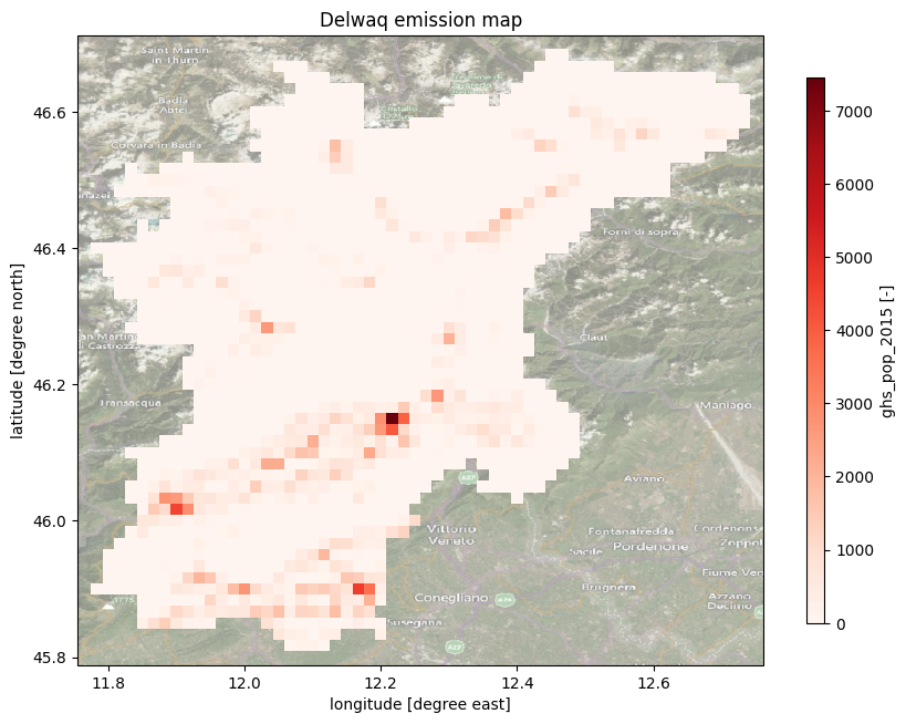
Plot model emission maps

Here we plot the model grid (emission grids).

#List of available emission data in the model
print(f"Available static data: {list(mod.grid.keys())}")

Available static data: ['river', 'slope', 'streamorder', 'SoilThickness', 'porosity', 'ptiddown', 'monareas', 'ghs_pop_2015', 'gdp_world']

Use the code below to plot the different available emission data. You can also change the colors by using available colormaps from matplotlib.

# Edit the lines below to change the emission map and its colormap
emissionmap = 'ghs_pop_2015'
colormap = 'Reds'

#Load the emission map
da = mod.grid[emissionmap].raster.mask_nodata()
da.attrs.update(long_name=emissionmap, units='-')

#Plot
# we assume the model maps are in the geographic CRS EPSG:4326
proj = ccrs.PlateCarree()
# adjust zoomlevel and figure size to your basis size & aspect
zoom_level = 10
figsize=(10, 8)

# initialize image with geoaxes
fig = plt.figure(figsize=figsize)
ax = fig.add_subplot(projection=proj)
extent = np.array(da.raster.box.buffer(0.02).total_bounds)[[0, 2, 1, 3]]
ax.set_extent(extent, crs=proj)

# add sat background image
ax.add_image(cimgt.QuadtreeTiles(), zoom_level, alpha=0.5)

## plot emission map
cmap = plt.cm.get_cmap(colormap)
kwargs = dict(cmap=cmap)
# plot 'normal' elevation
da.plot(transform=proj, ax=ax, zorder=1, cbar_kwargs=dict(aspect=30, shrink=.8), **kwargs)

ax.xaxis.set_visible(True)
ax.yaxis.set_visible(True)
ax.set_ylabel(f"latitude [degree north]")
ax.set_xlabel(f"longitude [degree east]")
_ = ax.set_title(f"Delwaq emission map")