Mesh2d Basics

This is the basic introduction for using the meshkernel library.

meshkernel can be used for creating and manipulating various kinds of meshes.

The most common case deals with unstructured, two-dimensional meshes which is why this tutorial focuses on these.

At the very beginning, the necessary libraries have to be imported.

import matplotlib.pyplot as plt
import numpy as np

from meshkernel import GeometryList, MakeGridParameters, MeshKernel, ProjectionType

meshkernel provides a set of convenience methods for creating common meshes.

We use the curvilinear_compute_rectangular_grid method to create a simple curvilinear grid. You can look at the documentation in order to find all its parameters.

mk = MeshKernel()

make_grid_parameters = MakeGridParameters()
make_grid_parameters.num_columns = 3
make_grid_parameters.num_rows = 2
make_grid_parameters.angle = 0.0
make_grid_parameters.origin_x = 0.0
make_grid_parameters.origin_y = 0.0
make_grid_parameters.block_size_x = 1.0
make_grid_parameters.block_size_y = 1.0

mk.curvilinear_compute_rectangular_grid(make_grid_parameters)

We convert the curvilinear grid to an unstructured mesh and get the resulting mesh2d

mk.curvilinear_convert_to_mesh2d()

mesh2d_input = mk.mesh2d_get()

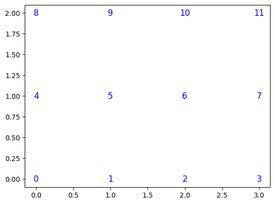
Mesh2D has three mandatory attributes, which are enough to fully describe any unstructured mesh.

The first two are node_x and node_y. They are one-dimensional double arrays, which describe the position of the nodes as can be seen below.

fig, ax = plt.subplots()

# Plot white points only for scaling the plot
ax.plot(mesh2d_input.node_x, mesh2d_input.node_y, "ow")

# Numbering the nodes
for i in range(mesh2d_input.node_x.size):
    ax.annotate(
        int(i),
        xy=(mesh2d_input.node_x[i], mesh2d_input.node_y[i]),
        ha="center",
        va="center",
        fontsize=12,
        color="blue",
    )

The third mandatory attribute is edge_nodes. It describes the indices of the nodes that make up the edges.

Two indices describe one edge. So in our case the indices 0-4, 1-5, 2-6, … each describe one edge.

mesh2d_input.edge_nodes

array([ 0,  4,  1,  5,  2,  6,  3,  7,  4,  8,  5,  9,  6, 10,  7, 11,  0,
        1,  1,  2,  2,  3,  4,  5,  5,  6,  6,  7,  8,  9,  9, 10, 10, 11])

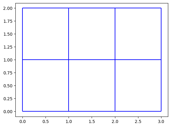
With all three parameters together we can plot the mesh.

fig, ax = plt.subplots()
mesh2d_input.plot_edges(ax, color="blue")

In order to interact with the meshkernel library, we create a new instance of the MeshKernel class.

The projection parameter of its constructor describes whether the mesh is cartesian (ProjextionType.CARTESIAN) or spherical (ProjextionType.SPHERICAL).

mk = MeshKernel(projection=ProjectionType.CARTESIAN)

Each instance holds it own state. This state can be accessed with the corresponding getter and setter methods.

mk.mesh2d_set(mesh2d_input)

mesh2d_output_0 = mk.mesh2d_get()

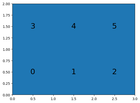
We have now set mesh2d and immediately got it again, without asking meshkernel to execute any operations in between.

After we set the mesh2d, meshkernel calculated the face data and edge coordinates.

fig, ax = plt.subplots()
mesh2d_output_0.plot_faces(ax)

# Draw face index at the face's center
for face_index, (face_x, face_y) in enumerate(
    zip(mesh2d_output_0.face_x, mesh2d_output_0.face_y)
):
    ax.text(face_x, face_y, face_index, ha="center", va="center", fontsize=22)

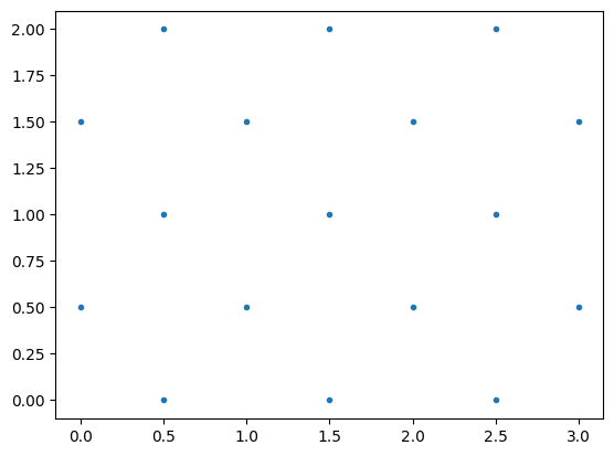
meshkernel also searches for the middle point of edges and adds them as parameters to the Mesh2D class.

fig, ax = plt.subplots()
ax.plot(mesh2d_output_0.edge_x, mesh2d_output_0.edge_y, ".");

Until now everything looked structured, so let us add a few nodes to change that.

node_index_0 = mk.mesh2d_insert_node(4.0, 1.5)
node_index_1 = mk.mesh2d_insert_node(4.0, 2.5)

We also have to connect our nodes, otherwise meshkernel will garbage collect them.

edge_index_0 = mk.mesh2d_insert_edge(7, node_index_0)
edge_index_1 = mk.mesh2d_insert_edge(node_index_0, node_index_1)
edge_index_3 = mk.mesh2d_insert_edge(node_index_1, 11)

Let us get the new state.

mesh2d_output_1 = mk.mesh2d_get()

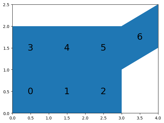
If we plot the output, we can also see that meshkernel immediately found a new face.

fig, ax = plt.subplots()
mesh2d_output_1.plot_faces(ax)

# Draw face index at the face's center
for face_index, (face_x, face_y) in enumerate(
    zip(mesh2d_output_1.face_x, mesh2d_output_1.face_y)
):
    ax.text(face_x, face_y, face_index, ha="center", va="center", fontsize=22)

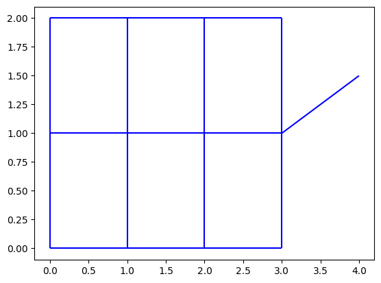
We can also delete nodes.

mk.mesh2d_delete_node(node_index_1)
mesh2d_output_2 = mk.mesh2d_get()

We are back to six faces, but one hanging edge remains.

fig, ax = plt.subplots()
mesh2d_output_2.plot_edges(ax, color="blue")

Quite often, hanging edges are unwanted. That is why meshkernel provides methods to deal with them. For once we can it can count hanging edges.

hanging_edges = mk.mesh2d_get_hanging_edges()
assert hanging_edges.size == 1

meshkernel can also find and delete them.

mk.mesh2d_delete_hanging_edges()
mesh2d_output_3 = mk.mesh2d_get()

After we have deleted the hanging edges, we are back at the original state.

fig, ax = plt.subplots()
mesh2d_output_3.plot_edges(ax, color="blue")