Pre-processing example (with HYDROLIB-core)#

If you prefer to interact with a Python script instead, you can convert this notebook to *.py with jupyter nbconvert --to script preprocessing_example_hydrolib.ipynb.

[1]:

# this notebook does not run in binder, since the data is not yet available online
import os
import numpy as np
import matplotlib.pyplot as plt
plt.close('all')
import dfm_tools as dfmt
import hydrolib.core.dflowfm as hcdfm

[2]:

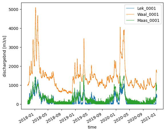
# load bc-file as HYDROLIB-core ForcingModel object (timeseries)
file_bc = r'p:\archivedprojects\11208053-004-kpp2022-rmm1d2d\C_Work\09_Validatie2018_2020\dflowfm2d-rmm_vzm-j19_6-v2d\boundary_conditions\rmm_rivdis_meas_20171101_20210102_MET.bc'
forcingmodel_object = hcdfm.ForcingModel(file_bc)

fig, ax = plt.subplots(figsize=(10,4))
# loop over three timeseries in bcfile/ForingModel
for iFO, forcingobj in enumerate(forcingmodel_object.forcing):
    forcing_xr = dfmt.forcinglike_to_Dataset(forcingobj, convertnan=True)
    forcing_xr['dischargebnd'].plot(ax=ax, label=forcing_xr['dischargebnd'].attrs['locationname'], linewidth=0.8)
ax.legend(loc=1)

[2]:

<matplotlib.legend.Legend at 0x217623de120>

../_images/notebooks_preprocessing_example_hydrolib_2_1.png

[3]:

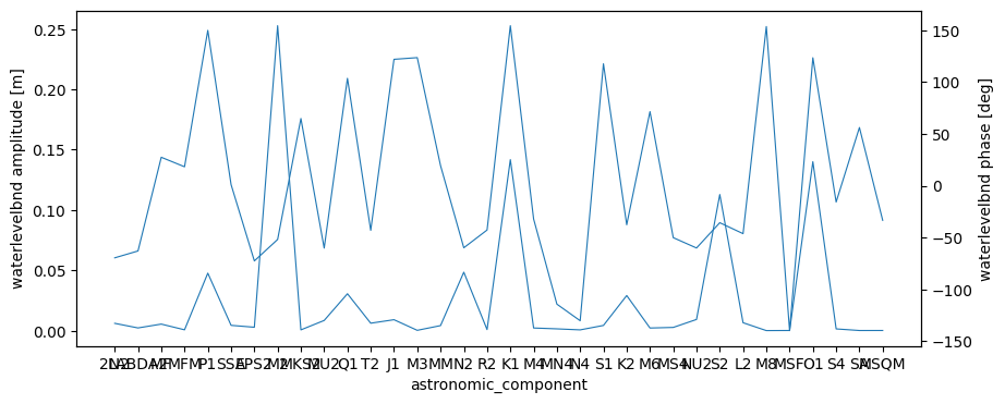
# load bc-file as HYDROLIB-core ForcingModel object (tidal components)
file_bc = r'p:\archivedprojects\11208154-002-haixia\02-hydrodynamics\02_Model_set_up\02_Make_forcing\FES2014\New_bnd_lines_2022\bc_South_v2.bc'
forcingmodel_object = hcdfm.ForcingModel(file_bc)

fig, ax = plt.subplots(figsize=(16,4))
ax2 = ax.twinx()
forcing_xr = dfmt.forcinglike_to_Dataset(forcingmodel_object.forcing[0], convertnan=True)
forcing_xr['waterlevelbnd amplitude'].plot(ax=ax)
forcing_xr['waterlevelbnd phase'].plot(ax=ax2)

[3]:

[<matplotlib.lines.Line2D at 0x217623ddfd0>]

../_images/notebooks_preprocessing_example_hydrolib_3_1.png

[4]:

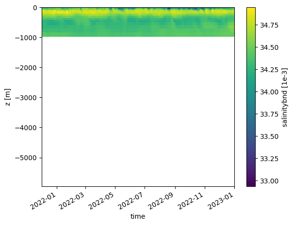
# load bc-file as HYDROLIB-core ForcingModel object (3D timeseries)
file_bc = r'p:\archivedprojects\11208154-002-haixia\02-hydrodynamics\02_Model_set_up\02_Make_forcing\CMEMS\bc_2022\South_v2\nonan\salinitybnd_bc_South_v2_CMEMS.bc'
forcingmodel_object = hcdfm.ForcingModel(file_bc)

fig, ax = plt.subplots(figsize=(10,4))
forcing_xr = dfmt.forcinglike_to_Dataset(forcingmodel_object.forcing[0], convertnan=True)
forcing_xr['salinitybnd'].T.plot(ax=ax)

[4]:

<matplotlib.collections.QuadMesh at 0x21762744b30>

../_images/notebooks_preprocessing_example_hydrolib_4_1.png

[5]:

# load bc-file as HYDROLIB-core ForcingModel object (3D timeseries vector)
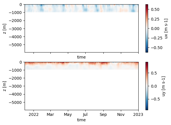
file_bc = r'p:\archivedprojects\11208154-002-haixia\02-hydrodynamics\02_Model_set_up\02_Make_forcing\CMEMS\bc_2022\South_v2\nonan\uxuy_bc_South_v2_CMEMS.bc'
forcingmodel_object = hcdfm.ForcingModel(file_bc)

fig, (ax1,ax2) = plt.subplots(2,1, figsize=(10,4), sharex=True, sharey=True)
forcing_xr = dfmt.forcinglike_to_Dataset(forcingmodel_object.forcing[0], convertnan=True)
forcing_xr['ux'].T.plot(ax=ax1)
forcing_xr['uy'].T.plot(ax=ax2)

[5]:

<matplotlib.collections.QuadMesh at 0x21776c2baa0>

../_images/notebooks_preprocessing_example_hydrolib_5_1.png

[6]:

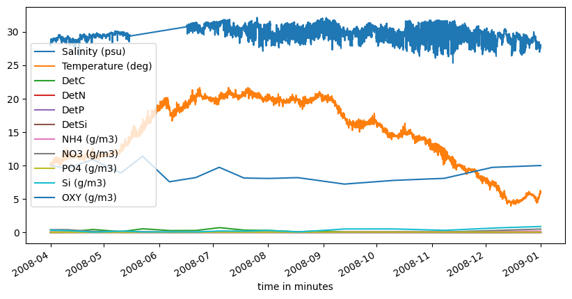
# load tim-file with HYDROLIB-core
file_tim = r'p:\archivedprojects\11206811-002-d-hydro-grevelingen\simulaties\Jaarsom2017_dfm_006_zlayer\boundary_conditions\hist\jaarsom_2017\sources_sinks\FlakkeeseSpuisluis.tim'
data_tim = hcdfm.TimModel(file_tim)
refdate = '2007-01-01'
tim_pd = dfmt.TimModel_to_DataFrame(data_tim, parse_column_labels=True, refdate=refdate)
tim_pd_sel = tim_pd.loc["2008-03":]
fig, ax = plt.subplots(figsize=(10,5))
tim_pd_sel.iloc[:, 1:12].plot(ax=ax)

[6]:

<Axes: xlabel='time in minutes'>

../_images/notebooks_preprocessing_example_hydrolib_6_1.png

[7]:

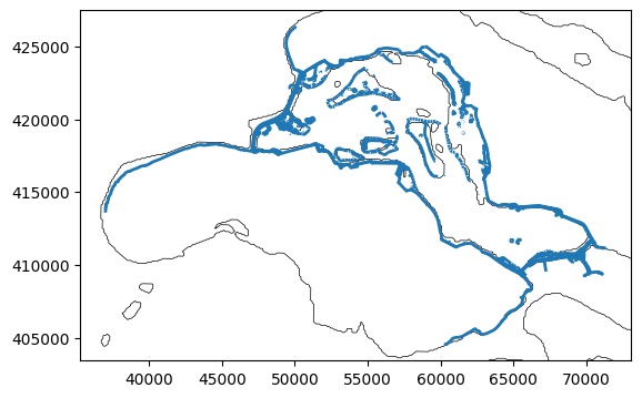
# load pol/pli/ldb file WITH HYDROLIB-core
file_pli = r'p:\archivedprojects\11205259-006-d-hydro-grevelingen\2Dh\model\2002\geometry\structures\Grevelingen-FM_BL_fxw.pliz'
polyfile_object = hcdfm.PolyFile(file_pli)
gdf_polyfile = dfmt.PolyFile_to_geodataframe_linestrings(polyfile_object,crs='EPSG:28992')
ax = gdf_polyfile.plot(linewidth=2)
dfmt.plot_coastlines(res='f', crs="EPSG:28992")

#get extents of all objects in polyfile
pol_bounds = gdf_polyfile.geometry.bounds
print("polygon_bounds:", pol_bounds['minx'].min(),pol_bounds['maxx'].max(),pol_bounds['miny'].min(),pol_bounds['maxy'].max())

>> reading coastlines: 1.75 sec
polygon_bounds: 36990.7701 71389.8071 404513.333 426415.3429

../_images/notebooks_preprocessing_example_hydrolib_7_1.png

[8]:

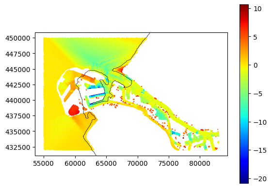
# load xyz data with HYDROLIB-core
file_xyz = r'p:\archivedprojects\11206813-006-kpp2021_rmm-2d\C_Work\31_RMM_FMmodel\geometry_j19_6-v2\rmm_vzm-j19_6-v2b_initial_water_level.xyz'
data_xyz = hcdfm.XYZModel(file_xyz)
fig,ax = plt.subplots()
xyz_gpd = dfmt.pointlike_to_geodataframe_points(data_xyz, crs="EPSG:28992")
xyz_gpd_sel = xyz_gpd.cx[55000:83000, 432000:450000]
xyz_gpd_sel.plot(ax=ax, column='z', markersize=0.5, cmap='jet', legend=True)
dfmt.plot_coastlines(res='f', crs="EPSG:28992")

>> reading coastlines: 0.80 sec

../_images/notebooks_preprocessing_example_hydrolib_8_1.png

[9]:

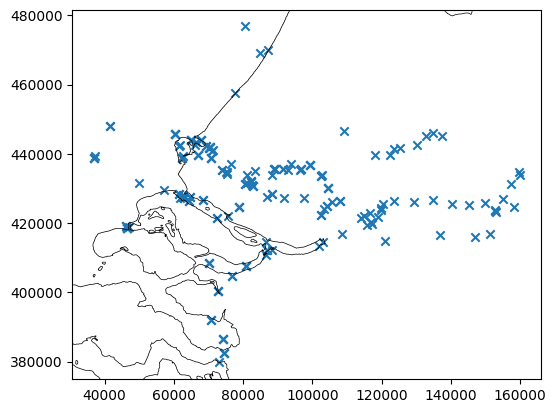
# load xyn data with HYDROLIB-core
file_xyn = r'p:\archivedprojects\11206813-006-kpp2021_rmm-2d\C_Work\31_RMM_FMmodel\geometry_j19_6-v2\output_locations\rmm_vzm-j19_6-v2b_3_measurement_obs.xyn'
data_xyn = hcdfm.XYNModel(file_xyn)
data_xyn_gpd = dfmt.pointlike_to_geodataframe_points(data_xyn, crs="EPSG:28992")
data_xyn_gpd.plot(marker='x')
dfmt.plot_coastlines(res='f', crs="EPSG:28992")

>> reading coastlines: 1.42 sec

../_images/notebooks_preprocessing_example_hydrolib_9_1.png

[10]:

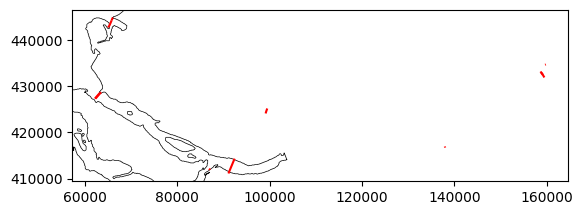
# load _crs.pli data with HYDROLIB-core
file_crs = r'p:\archivedprojects\11206813-006-kpp2021_rmm-2d\C_Work\31_RMM_FMmodel\geometry_j19_6-v2\cross_sections\rmm_vzm-j19_6-v2b_3_measurement_crs.pli'
data_crs = hcdfm.PolyFile(file_crs) # works with polyfile
polyobject_gpd = dfmt.PolyFile_to_geodataframe_linestrings(data_crs, crs="EPSG:28992")
polyobject_gpd.plot(color='r')
dfmt.plot_coastlines(res='f', crs="EPSG:28992")

>> reading coastlines: 1.13 sec

../_images/notebooks_preprocessing_example_hydrolib_10_1.png

[11]:

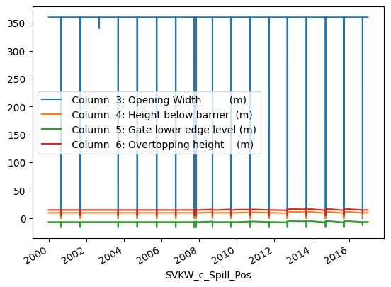
# load tekal file WITH HYDROLIB-core
file_pli = r'p:\archivedprojects\11205258-006-kpp2020_rmm-g6\C_Work\04_randvoorwaarden\keringen\Maeslantkering\Maeslant.tek'
polyfile_object = hcdfm.PolyFile(file_pli)
polyobject_pd = dfmt.tekalobject_to_DataFrame(polyfile_object.objects[0])
ax = polyobject_pd.plot()

../_images/notebooks_preprocessing_example_hydrolib_11_0.png

[ ]:

Pre-processing example (with HYDROLIB-core)#

This Page