Particle Tracking
Requirements
- Be sure QGIS version 3.40 or later is installed
- Be sure the QGIS-Tim plugin version 0.7.0 or later is installed (see installation for instructions).
- Be sure the
gistimversion 0.7.0 or later is installed (see installation for instructions). This is the Python package that connects QGIS-Tim to the timflow kernel.
Description
In this tutorial, we will show how to use the particle tracking feature of QGIS-Tim. This feature allows you to track the movement of particles in a groundwater flow field, which can be useful for understanding the flow paths and travel times of groundwater. We will use a simple example to demonstrate how to set up and run a particle tracking simulation using QGIS-Tim.
Area description
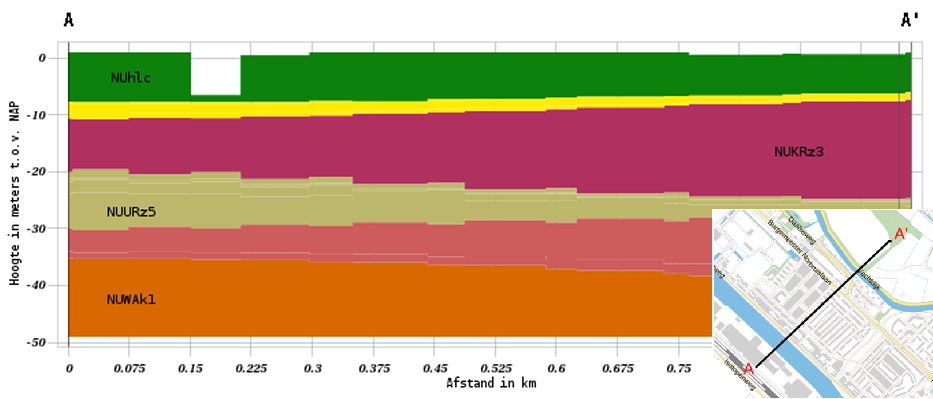
The area of interest is located in the Netherlands, near the city of Utrecht. The subsurface consists of a complex confining unit, followed by multiple sandy units, finally underlain by a clayey unit that acts as an aquitard. To keep things simple for this example, this clay layer is chosen as hydrogeological base. The area is bounded by a large canal, the Amsterdam-Rijn Kanaal (ARK), which is dug nearly through the confining unit, and a river, the Vecht.
Getting Started
- Launch QGIS
We start with the creation of a new QGIS project.
- From the main menu click on Project and select New.
The case in this tutorial is located in The Netherlands, so next we select the appropriate projection.
From the main menu click on Project and select Properties.
In the Properties window select the category CRS, search for “EPSG:28992” and you find “Amersfoort / RD New”. Select this option and click the Apply button, followed by the OK button to close the window.
Go to Project in the main menu, select Save As and select a folder and a file name for your project, e.g. “…\QGIS-Tim_Tutorial\particle_tracking.qgz”
Load the tutorial data
- First we’ll open the model which is part of the tutorial material
. Click on Model Manager, click Open and select ““./Zuilen_particle_tracking.gpkg”“.
This will load the model into the QGIS-Tim plugin. The model consists of a single 35 m thick sandy aquifer with a K of 10 m/d, bounded by two rivers and topped with a recharge area (Polygon Area Sink). The effect of the complex confined unit is accounted for in the resistances of the rivers in the model.
- Check the attribute tables of the aquifer, the two rivers, and the recharge area to see the parameters that are used in the model.
Let’s compute the groundwater head distribution in the model area.
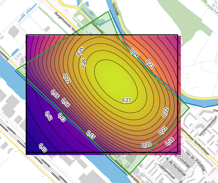
- Click on Results and click on Compute to compute the groundwater head distribution. This will open a black prompt window, please don’t close this! Otherwise, the computation will be interrupted. After the computation is finished, the groundwater head distribution will be visualized in the map canvas.
Forward Particle Tracking
Next, let’s release some particles in the model and track their movement.
Go to Elements and click the Particle Forward button. Provide a layer name in the prompt (e.g. “particle”) and click OK.
Select the “steady-state Particle Forward” on the left.
Click your right mouse button and select the Toggle Editing Mode (
 ).
).Click the Add Point Feature button (
 ) and click in the map canvas to add a particle. (TIP: For a nice result, place the particle near the maximum groundwater head.) You can add as many particles as you like, but for this tutorial we will add just one particle.
This will open a form to enter the attributes of the particle. Fill in the following values:
| parameter | value | unit | comment |
|---|---|---|---|
| fid | Autogenerate | [-] | ID is autogenerated by QGIS |
| Label | 1 | [-] | |
| z_start | -10 | [m MSL] | starting depth of the particle |
| max_horizontal_step | 10 | [m MSL] | maximum horizontal step size |
| max_vertical_step_fraction | 0.1 | [-] | maximum vertical step as fraction of layer thickness |
| nstep_max | 100 | [-] | maximum number of steps |
The latter three paramaters control the step size of the particle tracking. Decreasing the step size will increase the accuracy of the particle tracking, but also increase the computation time.
After filling in the attributes, click OK to save the particle.
Click on Results and then under Output select the Particle Pathlines checkbox.
Next press Compute again to compute the particle tracking results. After the computation is finished, the particle track will be visualized in the map canvas.
Note: When particles travel for a very long time, the amount of years might exceed the maximum of years allowed in the geopackage (9999 years) and an error will be thrown. In case this happens, you can decrease nstep_max to a lower value (e.g. 30) and recompute the particle tracking results.
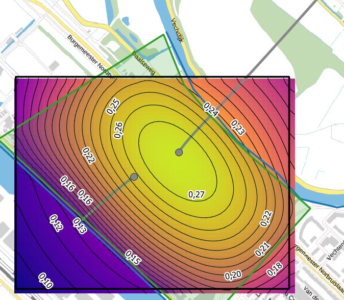
You’ll see that particles sent in the direction of the Vecht river (the river on the right) will not be captured by the river, whereas the particles sent in the direction of the Amsterdam Rijn Kanaal (ARK) will be captured by the canal (or at least are more likely to be captured).
Exercise: Investigate which River parameter causes this difference in behavior by comparing the attribute tables of the Vecht river and the Amsterdam Rijn Kanaal (ARK). Feel free to modify the parameters of the Vecht river and see how this affects the particle tracking results.
Travel times
Let’s also investigate the travel time of the particles. To do that, we’ll use the temporal controller of QGIS to animate the particle tracking results.
Let’s first make sure the temporal controller is enabled in QGIS. Go to View in the main menu, select Panels and make sure Temporal Controller is checked.
Open the Temporal Controller of QGIS (in the toolbar on top). (
 ).
).In the Temporal Controller panel click the green play button “Animated temporal navigation” on the right of the menu (
 ).
).
Navigation buttons appear which allow you to control the animation of the particle tracking results.
First, make sure the animation range is set properly by clicking the “Set to full range” button (
 ).
).Second, set the step size to 10 years. This means that the animation will show the particle positions every 10 years.
Next, click the play button to start the animation. You should see the particles moving as line segments. These line segments represent the pathlines of the particles within the selected time frame (of 10 years). This time frame is shown on top next to the temporal controller panel menu.
Note Depending on how you modified the model, you might want set the step size to a different value to be able to see the particle movement more clearly.
- Finally, you can view the tracelines of the particles in their entirety again by clicking the red cross button (“Turn off temporal navigation”) on the left of the menu ().
Note that closing the temporal controller panel will NOT turn off the temporal navigation.
Introducing a well
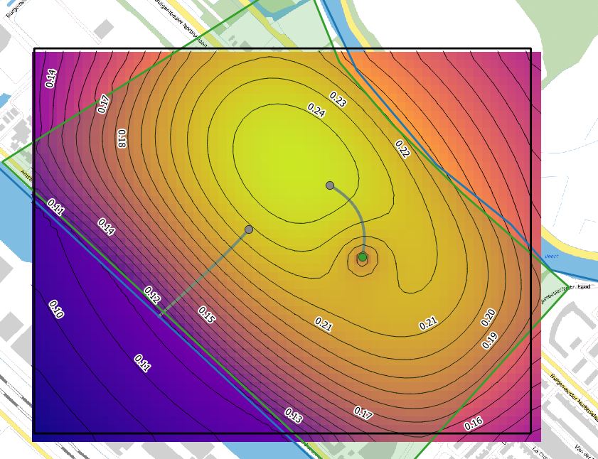
Let’s introduce a well in the model and investigate how this affects the particle’s direction and travel time.
(@): Place a well roughtly in the center of the model, by clicking Elements and then clicking the Well button.
Provide a name to the layer
Start editing your new well layer by clicking the Toggle Editing Mode button (
).Click the Add Point Feature button (
).This will open a form to enter the attributes of the well. Fill in the following values:
| parameter | value | unit | comment |
|---|---|---|---|
| fid | Autogenerate | [-] | ID is autogenerated by QGIS |
| discharge | 30 | [m3/d] | |
| radius | 0.1 | [m] | |
| resistance | 0 | [d] | |
| layer | 0 | [-] | |
| label | 1 | [-] |
After filling in the attributes, click OK to save the well.
Next press Compute again to compute the particle tracking results.
Investigate the capture zone
Let’s introduce trace some particles backwards to investigate the capture zone of the well.
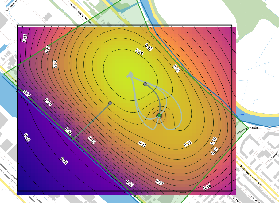
Click the Particle Backward button. Provide a layer name in the prompt (e.g. “capture_zone”) and click OK.
Select the “steady-state Particle Backward” on the left.
Click your right mouse button and select the Toggle Editing Mode button (
).Zoom in to the well you placed. Click the Add Point Feature button (
) and click in the map canvas to add a particles just around the well.This will open a form to enter the attributes of the particle. Fill in the following values:
| parameter | value | unit | comment |
|---|---|---|---|
| fid | Autogenerate | [-] | ID is autogenerated by QGIS |
| Label | 1 | [-] | |
| z_start | -40 | [m MSL] | starting depth of the particle |
| max_horizontal_step | 10 | [m MSL] | maximum horizontal step size |
| vertical_step_fraction | 0.1 | [-] | maximum vertical step as fraction of layer thickness |
| nstep_max | 50 | [-] | maximum number of steps |
After filling in the attributes, click OK to save the particle.
Next press Compute again to compute the particle tracking results.
Note: When particles travel for a very long time, the amount of years might exceed the maximum of years allowed in the geopackage (9999 years) and an error will be thrown. In case this happens, you can decrease nstep_max to a lower value (e.g. 30) and recompute the particle tracking results.