Usage
In Geomorphometry.jl we provide a set of tools to analyze and visualize the shape of the Earth. The package is designed to be fast, flexible, and easy to use. Moreover, we have implemented several algorithms for a common operation so that you can choose the one that best fits your needs.
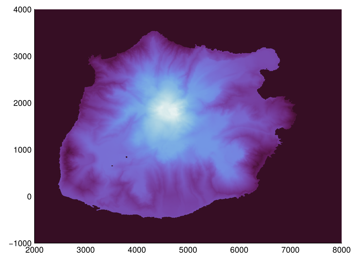
In these pages we will use the elevation model of Saba to showcase the different categories of operations that are available in Geomorphometry.jl.
Visualization
Visualization is done using the hillshade, multihillshade, and pssm functions. The first two shade the terrain by using a single or multiple light source(s) respectively, while pssm is a slope map exaggerated for human perception.
heatmap(hillshade(dtm))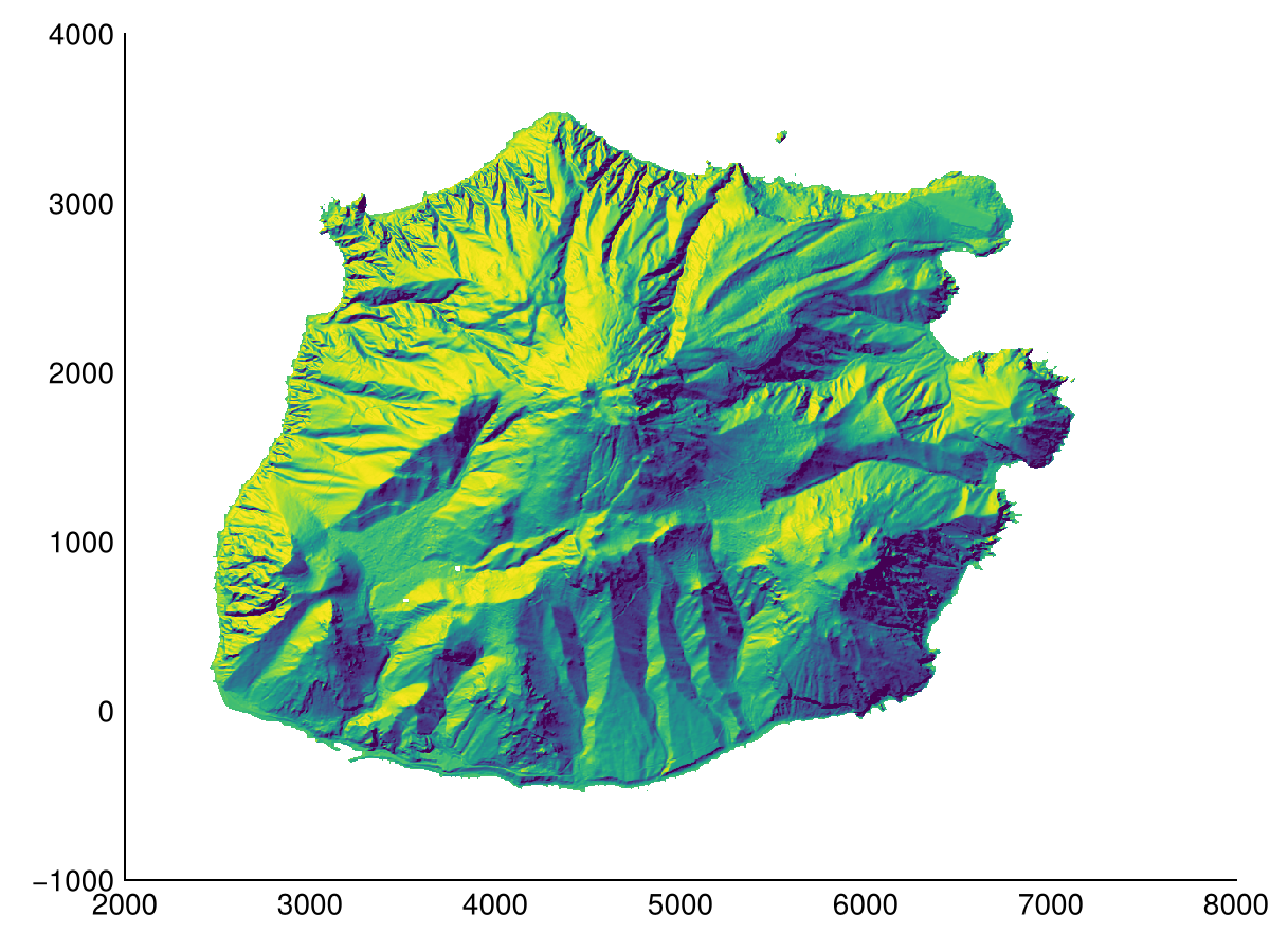
We can also overlay the pssm visualization on top of a colored aspect map.
f = heatmap(aspect(dtm); colormap=:curl)
heatmap!(pssm(dtm); colormap=Reverse(:greys), alpha=0.5)
f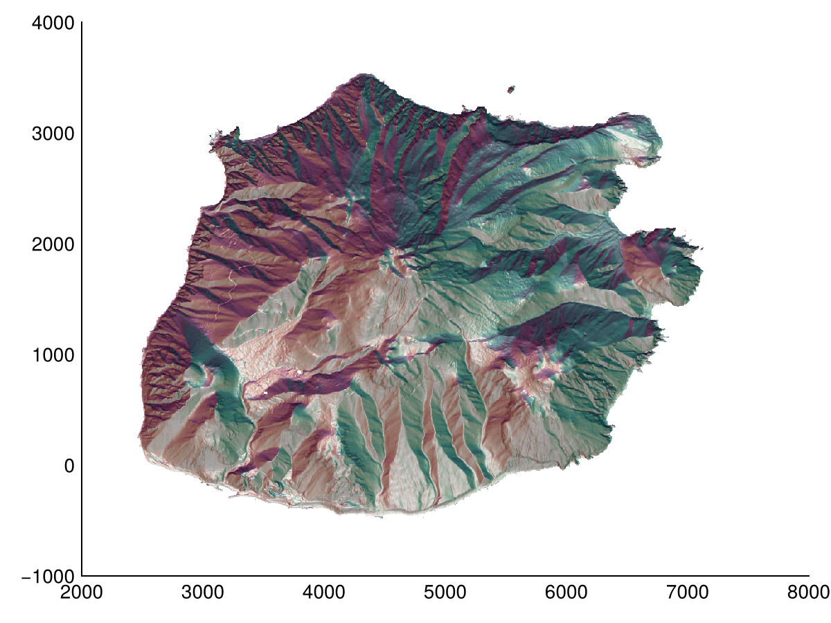
Derivatives
Common derivatives are implemented in Geomorphometry.jl. These include slope, aspect, and curvature. The latter is ill-defined, here we provide plan_curvature (also called projected contour curvature), profile_curvature (also called normal slope line curvature), and tangential_curvature (also called normal contour curvature). Note that functions here allow for a custom radius (but fixed positions, see X), as demonstrated for profile_curvature.
Slope
heatmap(slope(dtm; method=Horn()); colormap=:matter, colorrange=(0, 60))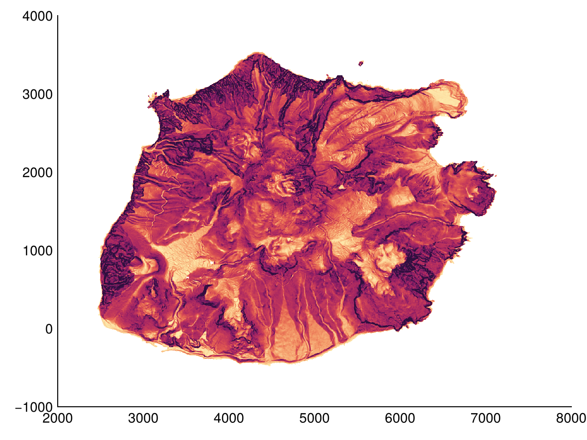
We can also determine the slope of the terrain along a specific direction.
heatmap(slope(dtm; method=Horn(), direction=0); colormap=:matter, colorrange=(-45, 45))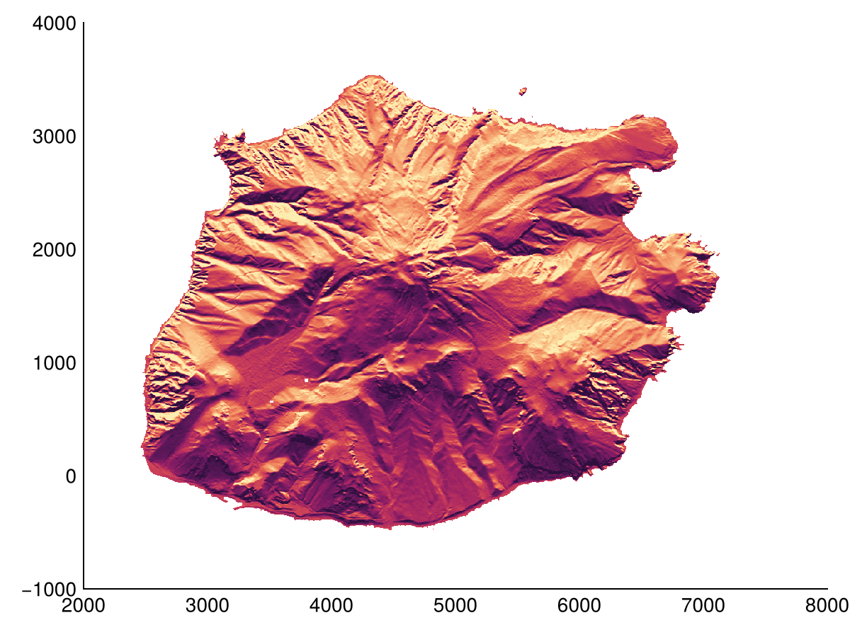
Aspect
heatmap(aspect(dtm; method=Horn()); colormap=:romaO)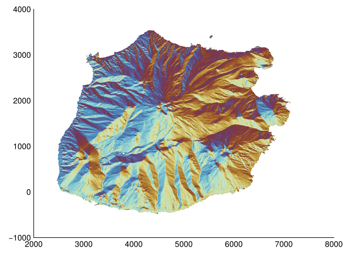
Curvature
heatmap(profile_curvature(dtm); colorrange=(-1,1), colormap=:tarn)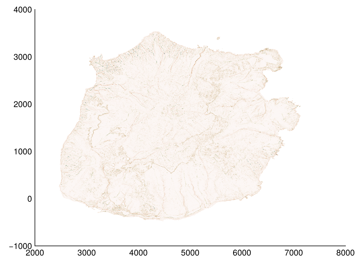
We can also determine the curvature of the terrain along a specific direction.
heatmap(laplacian(dtm, radius=1, direction=90); colorrange=(-1,1), colormap=:tarn)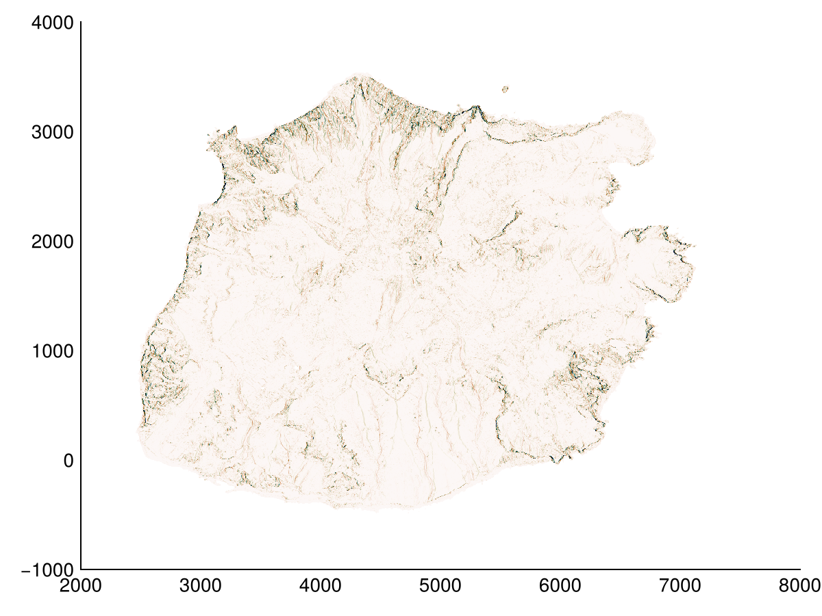
Relative position
There are several terrain descriptors that can be used to analyze the relative position of a point with respect to its neighbors. These include TPI, TRI, RIE, BPI, rugosity and roughness. Here we use BPI, but with a custom sized Window (from Stencils.jl). All these functions can be used with a custom window size.
heatmap(BPI(dtm, Geomorphometry.Annulus(5, 3)); colormap=:delta, colorrange=(-10,10))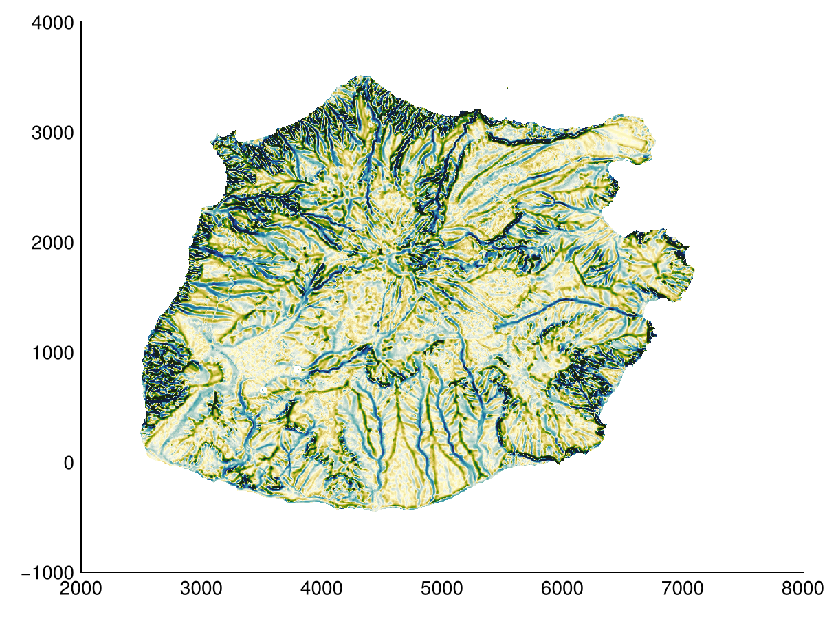
Hydrology
Hydrological operations are used to analyze the flow of water on the terrain. We provide filldepressions to fill depressions, and flowaccumulation to calculate the flow accumulation. Here we use flowaccumulation to calculate the flow accumulation. Note that the local drainage direction is also returned. By default the FD8 algorithm is used, but you can also use the D∞ or D8 algorithm by setting the method keyword argument to DInf() or D8().
acc, ldd = flowaccumulation(dtm; method=FD8(2))
heatmap(log10.(acc); colormap=:rain)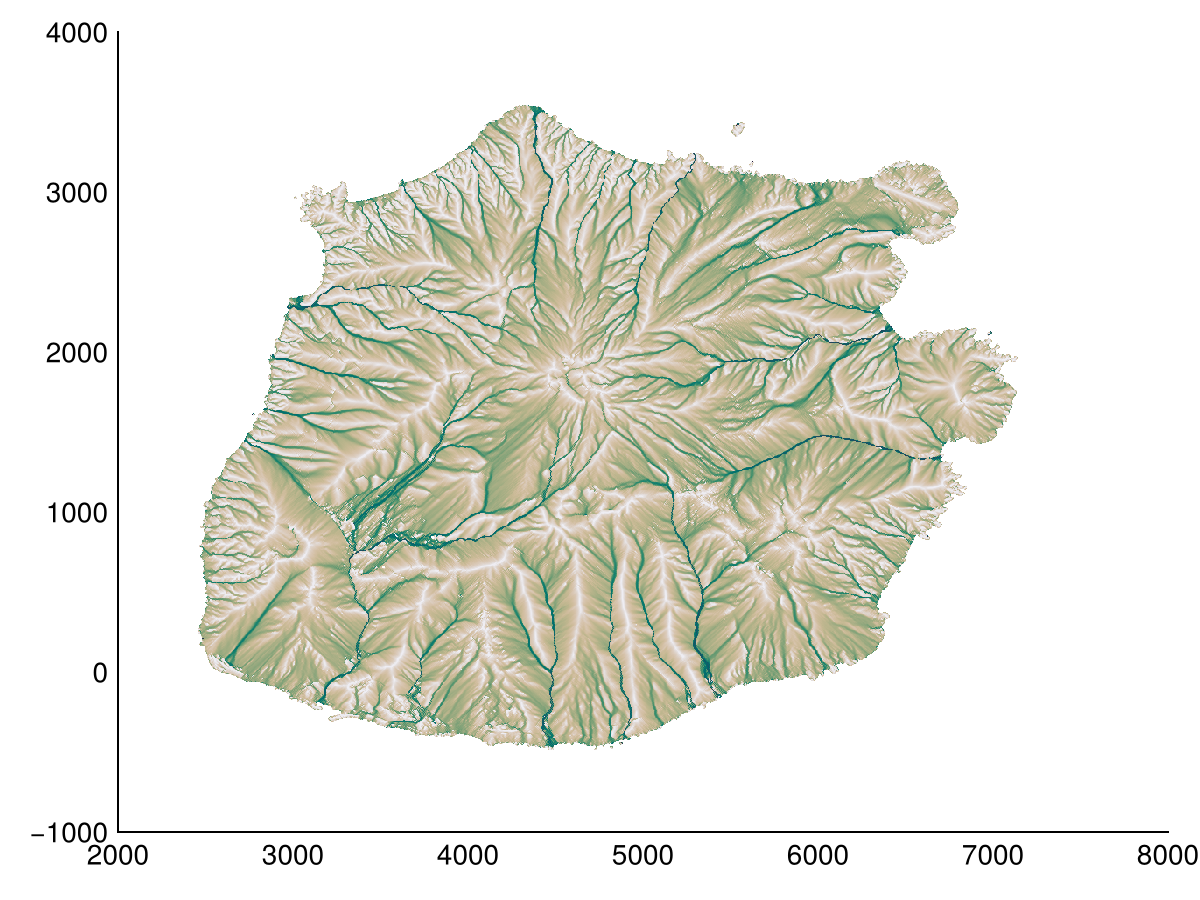
Combined with the previous analysis, we can calculate TWI and SPI indices. These indices are used to analyze the terrain's ability to accumulate water and the terrain's ability to store water respectively.
twi = TWI(dtm; method=FD8())
heatmap(twi; colormap=:tempo)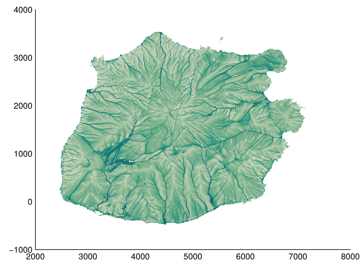
Terrain filters
While filters seem unrelated to the previously discussed methods, these are used to filter (rasterized) pointclouds i.e. surface models (DSM) to arrive at a terrain model (DTM). We provide pmf, smf, and skb filters. Here we use the pmf filter to remove elevations that do not pass the slope filter (normally vegetation and buildings).
B, flags = pmf(dsm, ωₘ = 15.0, slope = 0.2, dhₘ = 5.0, dh₀ = 0.3)
A = copy(dsm)
A[A .> B] .= NaN
heatmap(A)
Cost distance
Finally there are so-called cost distance functions. Instead of calculating a distance in the Euclidean sense, these functions calculate the cost of moving from one point to another, given a spatial varying cost. We provide a single spread function with multiple methods. The function takes starting points, an initial cost, and a cost (friction) map.
Here we use the top of the volcano as the starting point, and the squared slope as the cost map. We compare the Tomlin method with the Eikonal and Eastman methods. Eastman requires a high number of iterations to converge (even at 25 it's not enough), and is thus slower.
heatmap(spread(dtm .> 850, 0, slope(dtm).^2), colormap=:dense)