Concepts

In Geomorphometry.jl we provide a set of tools to analyse and visualize the shape of the Earth. The package is designed to be fast, flexible, and easy to use. It is built with the following concepts in mind:

Geospatially aware

With package extensions on GeoArrays.jl and Rasters.jl geospatial data is automatically handled to set the correct cellsize, even for geographical DEMs.

r = Raster("saba.tif")
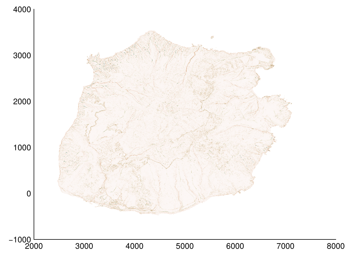
Geomorphometry.cellsize(r)

(5.0, -5.0)

heatmap(multihillshade(r))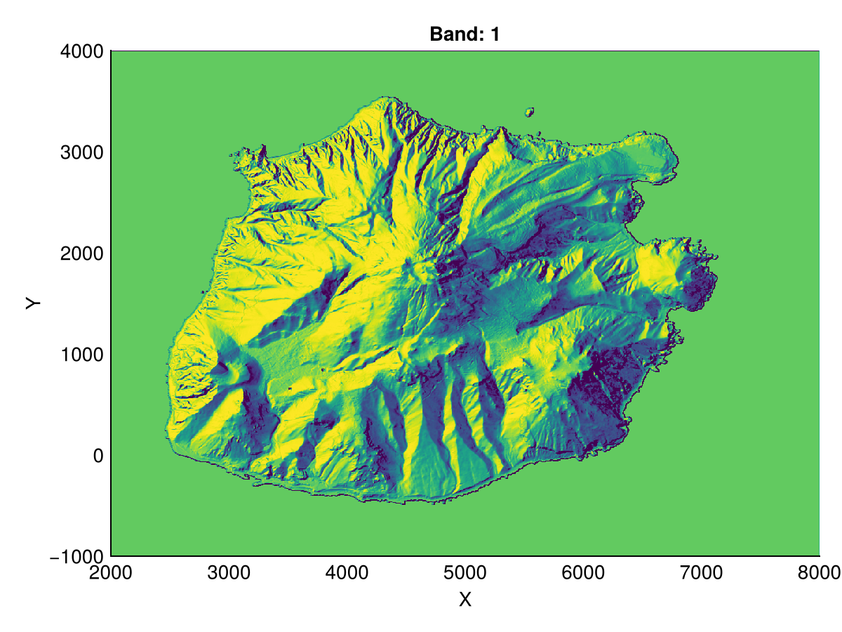

Multiple algorithms

We have implemented several algorithms for a common operation so that you can choose the one that best fits your needs. For example, the slope function has three methods: Horn, ZevenbergenThorne, and MaximumDownwardGradient, as shown in the Usage section.

Sometimes, as is the case for the FD8 algorithm, these methods take different parameters that influence the results. FD8 takes a p parameter that is used to weigh the flow direction, with higher powers resulting in less divergent flows (and thus more like D8).

acc, ldd = flowaccumulation(dtm; method=FD8(1))
heatmap(log10.(acc); colormap=:rain)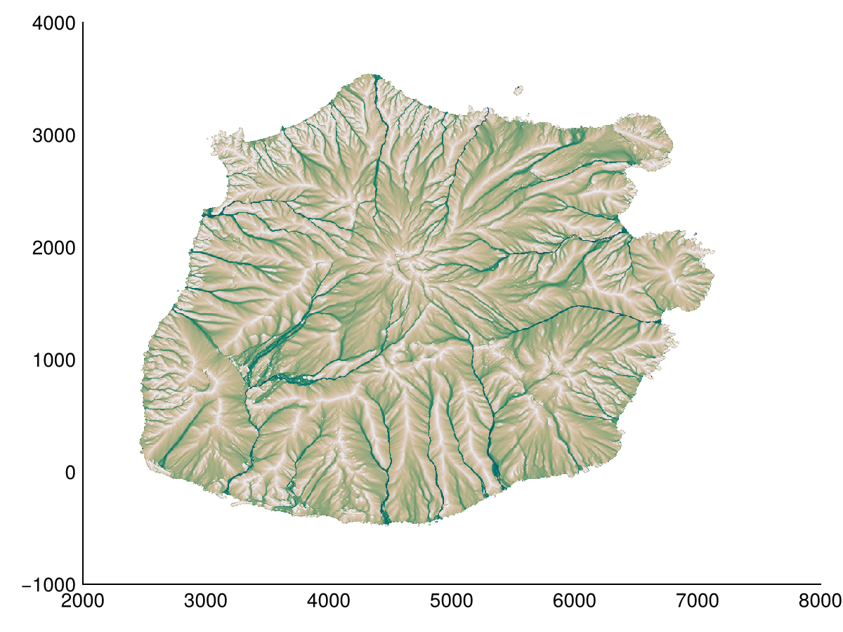

Multiple scales

Inspired by the excellent MultiScaleDTM package in R by Ilich et al. (2023), we have added multiscale options to some filters.

Relative terrain filters have a window keyword argument for a Stencil from Stencils.jl package.

Geomorphometry.Moore(1)

Stencils.Moore{1, 2, 8, Nothing}
█▀█
▀▀▀

heatmap(TPI(dtm, Geomorphometry.Moore(1)); colorrange=(0,25), colormap=:speed)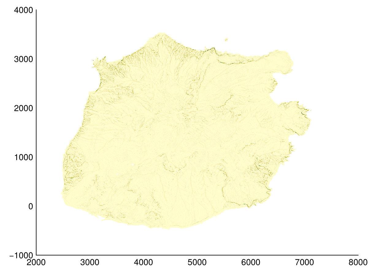

Other methods that require a specific type of window now take a radius kwarg, scaling said window.

Geomorphometry.scaled8nb(1)

Stencils.NamedStencil{(:Z1, :Z2, :Z3, :Z4, :Z5, :Z6, :Z7, :Z8, :Z9), ((-1, -1), (0, -1), (1, -1), (-1, 0), (0, 0), (1, 0), (-1, 1), (0, 1), (1, 1)), 1, 2, 9, Nothing}
███
▀▀▀

heatmap(profile_curvature(dtm, radius=1); colorrange=(-1,1), colormap=:tarn)